Deep Learning-Based High-Precision Depth Map Estimation from Missing Viewpoints for 360-Degree Digital Holography

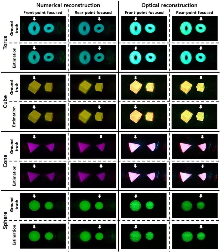
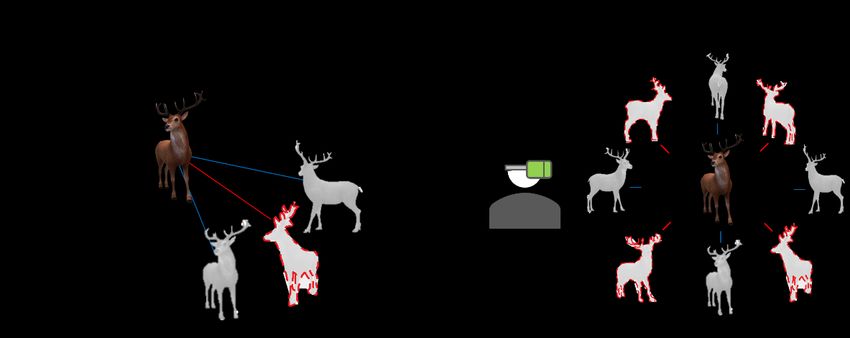
Deep Learning-Based High-Precision Depth Map
Estimation from Missing Viewpoints for 360-Degree
Digital Holography
Hakdong Kim1, Heonyeong Lim1, Minkyu Jee2, Yurim Lee3, Jisoo Jeong2,
Kyudam Choi2, MinSung Yoon4, *, and Cheongwon Kim5, **
1Department of Digital Contents, Sejong University, Seoul, 05006, South Korea
2Department of Software Convergence, Sejong University, Seoul, 05006, South Korea
3Department of Artificial Intelligence and Linguistic Engineering, Sejong University, Seoul, 05006, South Korea
4Communication & Media Research Laboratory, Electronics and Telecommunications Research Institute, Daejeon, 34129,

South Korea
5 Department of Software, Collage of Software Convergence, Sejong University, Seoul, 05006, South Korea
* msyoon@etri.re.kr
**wikim@sejong.ac.kr

ABSTRACT
In this paper, we propose a novel model to extract highly precise depth maps from missing viewpoints, especially
for generating holographic 3D content. These depth maps are essential elements for phase extraction, which is
required for the synthesis of computer-generated holograms (CGHs). The proposed model, called the holographic
dense depth, estimates depth maps through feature extraction, combining, up-sampling. We designed and prepared
a total of 8,192 multi-view images with resolutions of 640 × 360. We evaluated our model by comparing the
estimated depth maps with their ground truths using peak signal-to-noise ratio, accuracy, and root mean squared
error as performance measures. We further compared the CGH patterns created from estimated depth maps with
those from ground truths and reconstructed the holographic 3D image scenes from their CGHs. Both quantitative
and qualitative results demonstrate the effectiveness of the proposed approach.
Introduction
A depth map image represents information related to the distance between the camera’s viewpoint and the object’s
surface. It is reconstructed based on the original (RGB color) image and generally has a grayscale format. Depth
maps are used in three-dimensional computer graphics, such as three-dimensional image generation and computer-
generated holograms (CGHs). In particular, phase information, which is an essential element for CGHs, can be
acquired from depth maps [1, 2].
360-degree RGB images and their corresponding depth map image pairs are required to observe 360-degree digital
holographic content. If a specific location does not have a depth map (missing viewpoint), its corresponding
holographic 3D (H3D) scene will not be visible. Depth map estimation compensates for missing viewpoints and
contributes to the formation of realistic 360-degree digital hologram content. In this study, we propose a novel
method for learning depth information from captured viewpoints and estimating depth information from missing
viewpoints. The overall approach is shown in Fig. 1.

 Figure 1.

 1

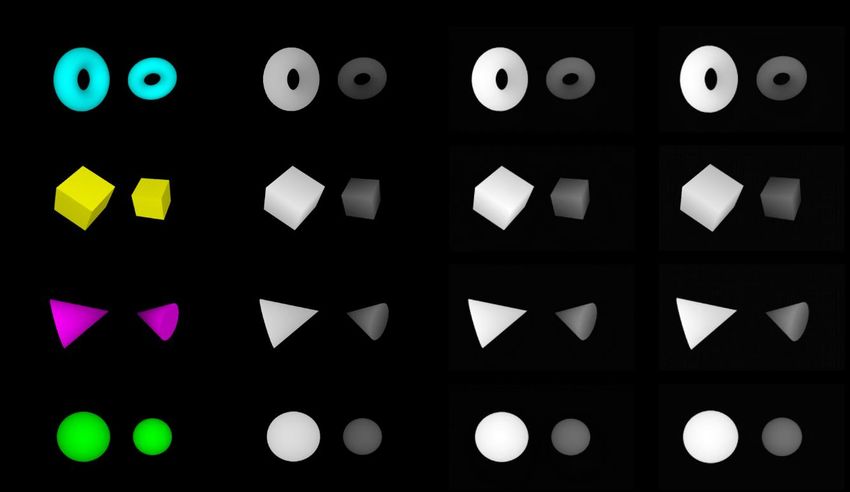
Many previous studies have estimated depth maps based on three distinct approaches. The first is the monocular
approach [3-10]. Battiato et al. [3] proposed the generation of depth maps using image classification. In this work,
digital images are classified as indoor, outdoor, and outdoor with geometric objects, with low computational costs.
Eigen et al. [4] proposed a convolutional neural network (CNN)-based model consisting of two different networks.
One estimates the global structure of the scene, whereas the other estimates the local information. Koch et al. [5]
studied the preservation of edges and planar regions, depth consistency, and absolute distance accuracy from a
single image. Other studies adopting conditional random fields [6-8], generative adversarial networks [9, 10], and
U-nets with an encoder-decoder structure have been introduced [11]. Alhashim et al. [12] applied transfer learning
to high-resolution depth map estimation, which we refer to as conventional dense depth (CDD) for the remainder
of this paper.
The second is the stereo approach, which uses a pair of left and right images [13]. In this method, depth maps are
estimated based on the disparity between two opposing viewpoints (two cameras). This approach follows the
intuition of recognizing the distance of an object the same way as the human visual system does. Self-supervised
learning, where the model estimates depth maps from stereo images using a monocular depth map of the left or
right image, has been applied to this type of approach [14].
The third approach estimate depth maps using multi-view images (more than two RGB images) [15-18]. Many of
them use the plane-sweep method [19], which is a basic geometry algorithm for finding intersecting line segments
[15-17]. Choi et al. [15] used CNNs for multi-view stereo matching, which combines the cost volumes with the
depth hypothesis in multi-view images. Im et al. [16] proposed an end-to-end model that learns a full plane-sweep
process, including the construction of cost volumes. Recently, Zhao et al. [17] proposed an asymmetric encoder-
decoder model that has improved accuracy for outdoor environments. Wang et al.’s work features a CNN for
solving the depth estimation problem on several image-pose pairs that are taken continuously while the camera is
moving [18]. All of the above studies can generate only a single depth image using multi-view RGB images.
To provide realistic holographic [20, 21], AR [22], or VR [23] content (see Fig. 1-b) to users, it is essential to
estimate as many highly precise depth maps as possible in a short time for each given narrow angular range.
Therefore, in this study, although we use the input data of multi-view RGB images, we do not adopt either
conventional stereo-view or multi-view methods because these methods use multiple RGB images as input to
output only a single depth map. Our model can generate new depth maps derived from new RGB images of the
missing viewpoints, as illustrated in (III) of Fig. 1-a. As a result, we can obtain 360-degree depth maps of objects
for realistic holographic or AR/VR content. Furthermore, we demonstrate the experimental results to test the
quality of the estimated depth maps by reconstructing holographic 3D scenes from the CGHs generated by the
estimated depth maps.

Results
Data Preparations
We first introduce a method that generates a 360-degree, multi-view RGB image-depth map pair dataset using the
Z-depth rendering function provided by 3D graphic software, Autodesk Maya 2018 [24]. Second, we present a
neural network architecture that estimates depth maps. Finally, the experimental results are discussed. In addition,
we also show the results of synthesizing CGHs, numerical reconstruction, and optical reconstruction using RGB
image-depth map pairs in the next section. In this study, a dataset of multi-view RGB image-depth map pairs was
generated using Z-depth rendering provided by Maya software. To extract the RGB image-depth map pairs in
Maya software, we devised two identical 3D objects located near the origin and a virtual camera with a light
source that shoots these two solid objects, so that the virtual camera could acquire depth difference information
between two solid figures during camera rotation around the origin. Depth measurements along the Z-direction
from the camera were made using a luminance depth preset supplied by the Maya software.
The virtual camera acquires 1024 pairs (for each shape of both RGB images and depth maps) while rotating 360-
degree around the axis of rotation. Shapes of 3D objects that we used for the study were a torus, cube, cone, and
sphere, as shown in Fig. 3. We use a total of 8,192 images for the experiments in this study. Among them, 4,096
are RGB images and the remaining 4,096 are depth map images. Both RGB images and depth map images are
classified into four shapes (torus, cube, cone, and sphere), each consisting of 1,024 views. When four kinds of
objects were learned at once, 60% of the total data were used for training, and 40% were used for testing
(estimation).

 2

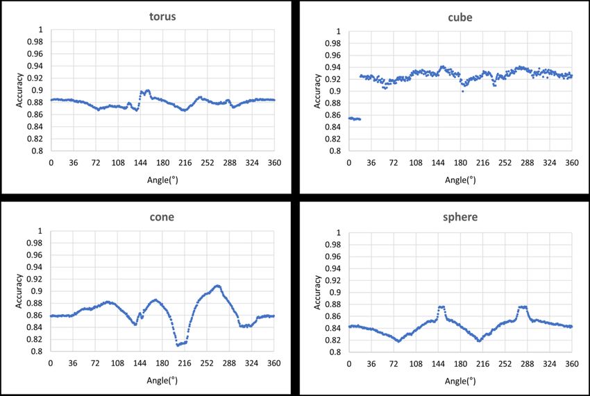
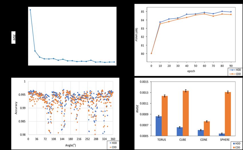
Quantitative Results
To quantitatively evaluate the performance of depth map estimation from the proposed model (HDD: holographic
dense depth), we first present a characteristic of the loss, mean squared error (MSE), averaged over all objects
during training for the HDD model in Fig. 2-a. Then, in the case of torus, we present the typical trends of peak
signal-to-noise (PSNR) of HDD and CDD in Fig. 2-b, where the x-axis represents the step number over 90 epochs.
In the case of torus, Fig. 2-c shows the distribution of accuracy (ACC) [25], indicating the similarity between the
ground truth depth map and the depth map estimated from HDD or CDD, where the x-axis represents the angular
degree corresponding to viewpoint (see Fig. 1). In addition, we present the RMSE from the HDD and CDD for
each object (Fig. 2-d).

 Figure 2.

We now introduce the loss function that we use in this study. The MSE was used as a loss function in the HDD
for more efficient gradient transfer. The MSE is defined as
 
 1
 = ∑( − ′)2
 
 =1
 (1)
which refers to the value measured by the pointwise operation of the difference between the depth value of the
estimated depth map ( ) and the depth value of the ground truth depth map ( ′ ), and n is the total number of
pixels. The quantitative metrics used in this study are as follows. The structural similarity (SSIM) [26] is defined
as

 (2 ′ + 1 )(2 ′ + 2 )
 =
 (2 2 + ′ 2 + 1 )( 2 + ′ 2 + 2 )
 (2)
which is commonly used to evaluate the similarity in visual quality (luminance, contrast, and structure) with the
original image, with as the average of ground truth(y); ′ the average of the estimated depth map(y’); 2
the variance of the ground truth(y); ′ 2 the variance of the estimated depth map(y’); 2 ′ the covariance of
ground truth(y) and estimated depth map(y’); and 1 , 2 are two variables for stabilizing the division with a weak
denominator, which is defined as

 1 = ( 1 )2 , 2 = ( 2 )2

 3

(3)
 
where L is the dynamic range of the pixel values (normally 2 − 1); and 1 and 2 are defined as
default values of 0.01 and 0.03, respectively. The SSIM of both models was approximately 0.9999. The PSNR is
defined as

 2
 = 10 
 
 (4)
which is defined via the MSE and s (maximal signal value of a given image), equal to 255 for the depth map image
of 8-bit gray levels used in this study. The ACC is defined as
 ∑ ( ∙ ′)
 =
 √[∑ 2 ][∑ ′2 ]
 (5)
where I is the depth value of pixels in the depth map image estimated by CDD or HDD, and I’ is the depth value
of pixels in the ground truth depth map image. When the estimation result and ground truth are identical, ACC =
1. However, note that if I = kI’ (k is scalar), ACC = 1, even if the estimation result and ground truth are different.
In addition, we use additional metrics that were used in prior studies [4, 12, 27, 28] as follows. Table 1 shows the
comparison results for these metrics for HDD and CDD.
 
 1 | − ′ |
 (Absolute Relative Error) = ∑
 ′
 =1
 (6)

 1 ( − ′ )2
 (Squared Relative Error) = ∑
 ′
 =1
 (7)

 1
 (Root Mean Squared Error) = √ ∑( − ′)2
 
 =1

 (8)

 1
 (Log Root Mean Squared Error) = √ ∑(LOG( ) − LOG( ′ ))2
 
 =1

 (9)

where is the depth value of a pixel in the estimated depth map, ′ is the depth value of a pixel in the ground
truth depth map, and n is the total number of pixels.

 4

Indicators
 a SSIM b PSNR (dB) c ACC
 Models Torus Cube Cone Sphere Torus Cube Cone Sphere Torus Cube Cone Sphere
 0.9933 0.9933 0.9928 0.9965
 HDD 0.9999 0.9999 0.9999 0.9999 84.95 84.42 84.90 85.03
 ±0.0040 ±0.0030 ±0.0037 ±0.0012
 0.9925 0.9934 0.9926 0.9959
 CDD 0.9999 0.9999 0.9999 0.9999 84.64 83.94 84.68 84.62
 ±0.0039 ±0.0027 ±0.0036 ±0.0013
 Indicators
 d Abs rel e Sq rel f RMSE
 Models Torus Cube Cone Sphere Torus Cube Cone Sphere Torus Cube Cone Sphere
 HDD 0.022 0.018 0.022 0.017 0.0058 0.0046 0.0058 0.0043 0.0009 0.0007 0.0006 0.0005
 CDD 0.019 0.017 0.016 0.017 0.0062 0.0052 0.0061 0.0047 0.0012 0.0013 0.0008 0.0013

 Indicators
 g LRMSE Time
 Resolution
 Models Torus Cube Cone Sphere Training Estimating
 HDD 0.0114 0.0117 0.0111 0.0110 17 h 0.18 s 640 × 360
 CDD 0.0116 0.0122 0.0113 0.0112 17 h 0.18 s 640 × 360
Table 1. Quantitative comparison of HDD (proposed model) and CDD (Using Nvidia Titan RTX ⅹ 8; a–c: higher is better; d–g: lower is
 better).

Qualitative Results
To qualitatively evaluate the depth map estimation performance of the HDD, we present samples of RGB
images, ground truths, and model estimation results from a viewpoint that is not used in training, as shown in
Fig. 3. (see Supplementary video 1)

 Figure 3.

According to the ground truth and the model's estimation result, it seems that HDD estimates the depth values of
the objects quite accurately. However, we can see that the part closer to the camera is slightly brighter than the
ground truth.

 5

Hologram image synthesis using depth estimation result
 Numerically reconstructed hologram images and optically reconstructed hologram images from the estimated
depth maps and ground truth depth maps are shown in Fig. 4. (The focused object is indicated with an arrow, see
Supplementary video 2-4)

 Figure 4.

The CGH was calculated from the RGB and depth map-based fast Fourier transform (FFT) algorithm, with either
a set of ground truth depth maps and RGB images or a set of estimated depth maps and corresponding RGB
images used as input for the FFT computational process of [29-30].
CGHs of 1,024 views were prepared for each solid figure, and a process of encoding called Lee’s scheme [29]
was adapted so that they could be represented on an amplitude-modulating spatial light modulator (SLM), that is,
a reflective LCoS (liquid crystal on silicon)-SLM. Lee’s encoding decomposes a complex-valued light field H( , )
into components with four real and non-negative coefficients, which can be expressed as

 ( , ) = 1 ( , ) 0 + 2 ( , ) /2 + 3 ( , ) + 4 ( , ) 3 /2
 (10)

 6

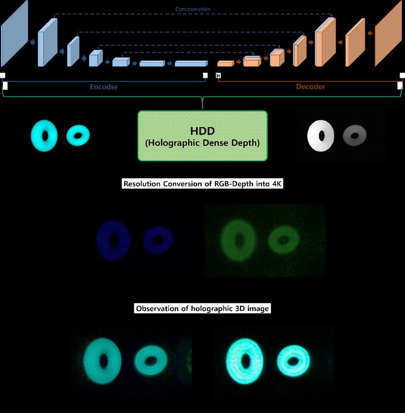
where at least two of the four coefficients ( ) are zero. The SLM that is used for optical reconstructions can
display an 8-bit grayscale, has a resolution of 3840 × 2160 pixels, an active diagonal length of 0.62”, and a pixel
pitch of 3.6 μm. A fibre-coupled, combined beam from RGB laser sources (wavelengths: 633 nm, 532 nm, and
488 nm of the MatchBox Laser Series) passes through an expanding/collimating optical device to supply coherent,
uniform illumination on the active area of the SLM. A field lens (focal length: f = 50 cm) was positioned just after
the LCoS-SLM, and experimental observation of the optically reconstructed images was performed using a DSLR
camera (Canon EOD 5D Mark III), whose lens was located within an observation window that was generated
near the focus of the field lens [30] (see Fig. 5). The results of camera-captured optical reconstructions and
numerical reconstructions from the synthesized CGHs are shown in Fig. 4. To prove the depth difference in real
3D space between two objects based on the prepared 360-degree holographic content, we demonstrate the
accommodation effect with optically realized holographic 3D scenes, by presentation to simultaneously indicate
the clear object and the blurred object in each picture when the camera lens is either on the rear focal plane or on
the front focal plane, as shown from each photograph in optical reconstruction’s column of Fig. 4.

 Figure 5.

When the holographic 3D images prepared from the depth map estimated using the proposed deep learning model
are observed, there is relative blurring in comparison with images prepared from the ground truth depth map. This
is because the minute difference between depth values of the two objects on the basis of estimation is not exactly
equal to the difference between the depth values of the two objects on the basis of reference (ground truth).
However, Fig. 4 shows that photographs of optically reconstructed scenes clearly support the accommodation
effect on holographic 3D images; when an object between two objects is within the camera’s focus, its
photographic image is very sharp, while an object that is out of focus is completely blurred.
In addition, in order to compare the CGH from the HDD estimation depth map with the CGH from the ground
truth depth map quantitatively, we carry out performance evaluation using the ACC, which is defined as

 ∑ , , ( ∙ ′)
 =
 √[∑ , , 2 ][∑ , , ′2 ]

 (11)
where I is the brightness of each color in the CGH image obtained using 2D RGB images and depth map images
estimated by HDD, and I' is the brightness of each color in the CGH image obtained using 2D RGB images and
ground truth depth map images. When the estimation result and ground truth are identical, or I = kI’ (k is a positive
scalar), ACC = 1. When a mismatch occurs between them, 0 ≤ ACC < 1. The comparison results are shown in
Fig. 6.

 7

Figure 6.

Discussion
In this paper, we proposed and demonstrated a novel CNN model that learns depth map estimation from missing
viewpoints, especially well-fit for holographic 3D. The proposed model, which we call HDD, uses MSE for better
depth map estimation performance in comparison with the CDD, which uses SSIM 90% and MSE 10% as the loss
function.
We designed and prepared 8,192 multi-view images with a resolution of 640 × 360. In the proposed model, HDD
estimated depth maps by extracting features and up-sampling. The weights were optimized using the MSE loss
function. For quantitative assessment, we compared the estimated depth maps from HDD with those from CDD
using the PSNR, ACC, RMSE. As shown in Fig. 2, the proposed HDD model is numerically superior to CDD in
terms of PSNR, ACC, and RMSE. In addition, as shown in Table 1, although HDD is numerically inferior to CDD
on the metrics of absolute relative error (abs rel), it is superior to CDD on the metrics of squared relative error
(sq rel) and LRMSE. We also compared fringe patterns created from the estimated depth maps with those created
from the ground truths. As shown in Fig. 6, the ACC values are approximately 0.84 to 0.92, depending on the
figures, which means that the fringe pattern made from the estimated depth map by the proposed model is
significantly similar to the fringe pattern made from the ground truth depth map.
The contributions of this study are as follows: First, we demonstrate the ability of our proposed HDD to learn and
produce depth map estimation with high accuracy from multi-view RGB images. Second, we prove the feasibility
of applying deep learning-based, estimated depth maps to synthesize CGHs, with which we can quantitatively
evaluate the degree of accuracy in the performance of our proposed model for holography. Third, we illustrate the
effectiveness of CGHs synthesized via the proposed HDD through direct numerical/optical observations of
holographic 3D images.
The limitations of the proposed model covered in this study are the minute residual images near the border area
of each object and the weak background noise in the estimated depth maps. To overcome these issues, one needs
to find approaches to place relatively large weights on these border areas and then enhance precision estimations
of these areas. It is also worth mentioning that the image resolution and extraction speed of deep learning-based
depth maps can be improved by adjusting the model’s parameters, such as filters and filter sizes, and then
optimizing the ratio of training/testing data. Moreover, we note that only the diffraction efficiency element, that
is, the direct observation of the reconstructed holographic 3D image, was used as a comparative measure for the
quality of the H3D image in this study. We plan to supplement this measure through further analysis, considering
parameters such as contrast ratio of intensity, clearness, and distortion to evaluate H3D images.

 8

Methods
The proposed depth map estimation model HDD consists of two components: the encoder and decoder, as shown
in Fig. 7. We adopt the dense depth (CDD) of Alhashim et al. [12]. The encoder performs feature extraction and
down-sampling of the input RGB images. The decoder performs up-sampling by concatenating the extracted
features based on the size of the RGB image. The weights for both components are optimized by a loss function
that minimizes the discrepancy between the ground truth and the estimated depth map. CDD learns and estimates
the depth from a single viewpoint. On the other hand, HDD learns depth from multiple viewpoints and estimates
the depth of viewpoints that are not used for training (new viewpoints). The CDD model used SSIM 90% and MSE
10% as the loss function, whereas the proposed HDD model only used MSE as the loss function. We also adopted
the CDD by utilizing bilinear interpolation in the up-sampling layer and ReLu as the activation function.
Consequently, we obtained better depth estimation results.

 Figure 7.

References
1. Brown, B. & Lohmann, A. Complex spatial filtering with binary masks. Appl. Opt. 5, 967-969 (1966).
2. Horisaki, R., Takagi, R. & Tanida, J. Deep-learning-generated holography. Appl. Opt. 57, 3859-3863
 (2018).
3. Battiato, S., Curti, S., La Cascia, M., Tortora, M.& Scordato, E. Depth map generation by image
 classification. Proc. SPIE 5302, Three-Dimensional Image Capture and Applications VI (2004).
4. Eigen, D., Puhrsch, C. & Fergus, R. Depth map prediction from a single image using a multi-scale deep
 network. Proc. Advances Neural Inf. Process. Syst., 2014, pp. 2366–2374. (2014).
5. Koch, T., Liebel, L., Fraundorfer, F. & Körner, M. Evaluation of CNN-based single-image depth estimation
 methods. European Conference on Computer Vision (ECCV) Workshops (2019).

 9

6. Li, B. & He, M. Depth and surface normal estimation from monocular images using regression on deep
 features and hierarchical CRFs. Proceedings of the IEEE Conference on Computer Vision and Pattern
 Recognition (CVPR), pp. 1119-1127 (2015).
7. Liu, F., Shen, C., Lin, G. & Reid, I. Learning depth from single monocular images using deep
 convolutional neural fields. IEEE PAMI, Vol. 38, pp. 2024-2039 (2015).
8. Wang, P. & Shen, X. Towards unified depth and semantic prediction from single image. Proceedings of the
 IEEE Conference on Computer Vision and Pattern Recognition (CVPR), pp. 2800-2809 (2015).
9. Lore, K. G., Reddy, K., Giering, M. & Bernal, E. A. Generative adversarial networks for depth map
 estimation from RGB video. Proceedings of the IEEE Conference on Computer Vision and Pattern
 Recognition (CVPR) Workshops, pp.1177-1185 (2018).
10. Aleotti, F., Tosi, F., Poggi, M. & Mattoccia, S. Generative adversarial networks for unsupervised
 monocular depth prediction. Proceedings of the European Conference on Computer Vision (ECCV)
 Workshops (2018).
11. Ronneberger, O., Fischer, P. & Brox, T. U-Net: convolutional networks for biomedical image
 segmentation. Medical Image Computing and Computer-Assisted Intervention – MICCAI 2015, pp.234-241
 (2015).
12. Alhashim, I. & Wonka, P. High quality monocular depth estimation via transfer learning. Preprint at
 https://arxiv.org/abs/1812.11941 (2018).
13. Alagoz, B. B. Obtaining depth maps from color images by region based stereo matching algorithms.
 OncuBilim Algor Syst Labs. Vol 8 (2009).
14. Martins, D., van Hecke, K. & de Croon, G. Fusion of stereo and still monocular depth estimates in a self-
 supervised learning context. 2018 IEEE International Conference on Robotics and Automation (ICRA),
 pages 849–856. (2018).
15. Choi, S., Kim, S., Park, K. & Sohn, K. Learning descriptor, confidence, and depth estimation in multi-view
 stereo. Proc. 2018 IEEE/CVF Conference on Computer Vision and Pattern Recognition Workshops, CVPRW
 2018, 389-395 (2018).
16. Im, S., Jeon, H., Lin, S. & Kweon, I. S. DPSNet: End-to-end deep plane sweep stereo. ICLR (2019).
17. Zhao, P. et al. MDEAN: Multi-view disparity estimation with an asymmetric network. Electronics. 9, 6,
 924 (2020).
18. Wang, K. & Shen, S. MVDepthNet: Real-time multiview depth estimation neural network. 2018
 International Conference on 3D Vision (3DV), IEEE. pages 248-257, (2018).
19. Wood, J. & Kim, S. Plane sweep algorithm. In: Shekhar, S., Xiong, H. (eds) Encyclopedia of GIS. Springer,
 Boston, MA. https://doi.org/10.1007/978-0-387-35973-1_989 (2008).
20. Shi, L., Li, B., Kim, C., Kellnhofer, P., Matusik, W. Towards real-time photorealistic 3D holography with
 deep neural networks. Nature. Vol. 591, pp. 234–239 (2021).
21. Nishitsuji, T., Kakue, T., Blinder, D., Shimobaba, T., Ito, T. An interactive holographic projection system
 that uses a hand-drawn interface with a consumer CPU. Sci Rep. Vol 11, 147 (2021).
22. Park, B.J., Hunt, S.J., Nadolski, G.J., Gade, T.P. Augmented reality improves procedural efficiency and
 reduces radiation dose for CT-guided lesion targeting: a phantom study using HoloLens 2. Sci Rep. Vol 10,
 18620 (2020).
23. Miller, M.R., Herrera, F., Jun, H., Landay, J.A., Bailenson, J.N. Personal identifiability of user tracking data
 during observation of 360-degree VR video. Sci Rep. Vol 10, 17404 (2020).
24. Maya 2018, Autodesk. https://www.autodesk.com/products/maya/overview
25. Hossein Eybposh, M., Caira, N. W., Atisa, M., Chakravarthula, P. & Pégard, N. C. DeepCGH: 3D
 computer-generated holography using deep learning. Opt. Express. 28, 26636-26650 (2020).
26. Wang, Z., Bovik, A. C., Sheikh H. R. & Simoncelli, E. P. Image quality assessment: from error visibility to
 structural similarity. IEEE Trans. Image Process. 13, no. 4, 600-612 (2004).
27. Wang, L., Famouri, M. & Wong, A. DepthNet Nano: A highly compact self-normalizing neural network for
 monocular depth estimation. Preprint at https://arxiv.org/abs/2004.08008 (2020).
28. Fu, H., Gong, M., Wang, C., Batmanghelich, K. & Tao, D. Deep ordinal regression network for monocular
 depth estimation. IEEE/CVF Conference on Computer Vision and Pattern Recognition, pp.2002-2011 (2018).
29. Lee, W. H. Sampled Fourier transform hologram generated by computer. Appl. Opt. Vol. 9, No. 3, pp. 639-
 644 (1970).
30. Yoon, M., Oh, K., Choo, H. & Kim, J. A spatial light modulating LC device applicable to amplitude-
 modulated holographic mobile devices. IEEE Trans. Industr. Inform. (INDIN). pp. 678-681 (2015).

 10

Figure captions

Figure 2. a Depth map estimation from missing viewpoint (III) using image set of captured viewpoints (I, II); b richer holographic 3D
content with estimated depth maps from missing viewpoints (III).

Figure 2. a Curve of the loss MSE averaged over all objects during training for the HDD model; b-d Comparison of HDD and CDD using
PSNR trend, ACC distribution with ground truth depth map for torus, RMSE difference for all objects after training.

Figure 3. Depth map comparison between ground truth, estimation result from HDD, and estimation result from CDD.

Figure 4. Result of numerical/optical reconstruction from CGHs using estimated depth map image and ground truth. (Focused object is
indicated by an arrow mark).

Figure 5. Geometry of the optical system for holographic 3D observation: a numerical simulation, and b its optical experiment setup.
Observer’s eye lens in a is located at the position of the focal length of the field lens, corresponding to the center of Fourier plane of the
optical holographic display b.

Figure 6. ACC trend for CGHs of torus, cube, cone, and sphere.

Figure 7. Pipeline for depth map estimation model and digital hologram reconstruction.

 11

Table

 Indicators
 a SSIM b PSNR (dB) c ACC
Models Torus Cube Cone Sphere Torus Cube Cone Sphere Torus Cube Cone Sphere
 0.9933 0.9933 0.9928 0.9965
 HDD 0.9999 0.9999 0.9999 0.9999 84.95 84.42 84.90 85.03
 ±0.0040 ±0.0030 ±0.0037 ±0.0012
 0.9925 0.9934 0.9926 0.9959
 CDD 0.9999 0.9999 0.9999 0.9999 84.64 83.94 84.68 84.62
 ±0.0039 ±0.0027 ±0.0036 ±0.0013
 Indicators
 d Abs rel e Sq rel f RMSE
Models Torus Cube Cone Sphere Torus Cube Cone Sphere Torus Cube Cone Sphere
 HDD 0.022 0.018 0.022 0.017 0.0058 0.0046 0.0058 0.0043 0.0009 0.0007 0.0006 0.0005
 CDD 0.019 0.017 0.016 0.017 0.0062 0.0052 0.0061 0.0047 0.0012 0.0013 0.0008 0.0013

 Indicators
 g LRMSE Time
 Resolution
Models Torus Cube Cone Sphere Training Estimating
 HDD 0.0114 0.0117 0.0111 0.0110 17 h 0.18 s 640 × 360
 CDD 0.0116 0.0122 0.0113 0.0112 17 h 0.18 s 640 × 360
Table 1. Quantitative comparison of HDD (proposed model) and CDD (Using Nvidia Titan RTX ⅹ 8; a–c: higher is better; d–g: lower is
 better).

 12