R 493 - Assessing financial stability risks from the real estate market in Italy: an update - Banca d'Italia
←
→
Page content transcription
If your browser does not render page correctly, please read the page content below
Questioni di Economia e Finanza
             (Occasional Papers)

             Assessing financial stability risks from the real estate
             market in Italy: an update

             by Federica Ciocchetta and Wanda Cornacchia
April 2019

                                                                          493
                                                                 Number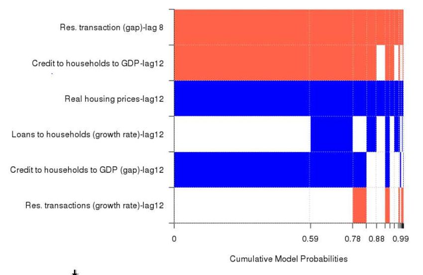

Questioni di Economia e Finanza
(Occasional Papers)

Assessing financial stability risks from the real estate
market in Italy: an update

by Federica Ciocchetta and Wanda Cornacchia

Number 493 – April 2019

The series Occasional Papers presents studies and documents on issues pertaining to
the institutional tasks of the Bank of Italy and the Eurosystem. The Occasional Papers appear
alongside the Working Papers series which are specifically aimed at providing original contributions
to economic research.

                 The Occasional Papers include studies conducted within the Bank of Italy, sometimes
in cooperation with the Eurosystem or other institutions. The views expressed in the studies are those of
the authors and do not involve the responsibility of the institutions to which they belong.

                 The series is available online at www.bancaditalia.it .

ISSN 1972-6627 (print)
ISSN 1972-6643 (online)

Printed by the Printing and Publishing Division of the Bank of Italy
ASSESSING FINANCIAL STABILITY RISKS FROM THE REAL ESTATE
                      MARKET IN ITALY: AN UPDATE

                                by Federica Ciocchetta* and Wanda Cornacchia*

                                                               Abstract
      We provide an update of the analytical framework to assess financial stability risks
arising from the real estate sector in Italy. The enhancement concerns the definition of a new
vulnerability indicator, measured in terms of the flow of total non-performing loans (NPLs)
and not, as done previously, in terms of bad loans only. We focus separately on households
(as an approximation for residential real estate, RRE) and on firms engaged in construction,
management and investment services in the real estate sector (as an approximation for
commercial real estate, CRE).
Two early warning models are estimated using the new vulnerability indicator for RRE and
CRE, respectively, as dependent variable. Both models exhibit good forecasting
performances: the median predictions fit well the new vulnerability indicators in out-of-
sample forecasts. Overall, models’ projections indicate that potential risks for banks
stemming from the real estate sector will remain contained in the next few quarters.

JEL Classification: C52, E58, G21.
Keywords: real estate markets, early warning models, bayesian model averaging, banking
crises.

                                                              Contents

1. Introduction.......................................................................................................................... 5
2. New vulnerability indicators for RRE and CRE.................................................................. 6
3. Early warning models .......................................................................................................... 9
4. Robustness checks ............................................................................................................. 13
5. Conclusions........................................................................................................................ 14
References .............................................................................................................................. 16

______________________________________
* Bank of Italy, DG for Economics, Statistics and Research, Financial Stability Directorate.

1. Introduction1
Systemic risks stemming from real estate markets have contributed significantly to financial
instability both in the past and in the recent financial crisis (Agnello and Schuknecht 2011). Crises
associated with credit crunches and housing price busts are indeed relatively frequent and
particularly harmful from a financial stability perspective since they are more protracted than other
recessions and may have severe repercussions on banks’ asset quality, banks’ failures and economic
growth (Claessens et al. 2008, Cerutti et al. 2015). Early identification of potential risks is
fundamental for macroprudential authorities in order to promptly implement the necessary
corrective policies.
In order to make a timely assessment of the risks for the Italian banking system arising from the real
estate sector, the Bank of Italy developed an analytical framework (Ciocchetta et al. 2016). This
framework consists of a broad set of indicators, describing the household sector, real estate market
and credit developments, and three early warning models (EWMs). EWMs are econometric models
designed to identify vulnerabilities in the run-up to a crisis (i.e. a situation where imbalances
accumulate, making the crisis more likely). They associate a crisis/non-crisis dummy variable or,
more generally, a vulnerability indicator with macro, real-estate and banks’ balance sheet variables
(see Alessi and Detken 2011, Babecky et al. 2012, Pirovano and Ferrari 2014, Ferrari et al. 2015,
Holopainen and Sarlin 2015). It is worth nothing that these methodologies do not aim to predict the
exact timing of a crisis, but rather to detect vulnerabilities that might lead to it (see Cornacchia and
Pirovano 2018). The modelling techniques used within the framework include both standard
methodologies used in the EWM literature, such as binary logit models, and models whose
application to this research field is relatively new, such as ordinal logit and Bayesian Model
Averaging (BMA) applied to linear regressions.
Since Italy has not experienced any real estate related banking crises, banks’ potential risks
stemming from the real estate sector are measured through the definition of a vulnerability
indicator. This describes the evolution of real estate exposures’ riskiness (expressed as the flow of
new bad loans)2 in terms of its impact on banks’ balance sheets (expressed as total capital and
reserves). The indicator, constructed for both the residential real estate (RRE) and commercial real
estate (CRE) sectors (proxied by firms engaged in construction, management and investment
services in the real estate sector), is then used as a dependent variable in the EWMs.3
This work focuses on the definition of a new vulnerability indicator for the banking system based
on the flow of total non-performing loans (NPLs) for both the RRE and CRE sectors. Previously the
vulnerability indicator was defined in terms of the flow of bad loans only, as estimation of EWMs
requires long time series and the flow of bad loans has been available on a quarterly basis since

1
  The views expressed herein are those of the authors and do not necessarily reflect those of the Bank of Italy or of the
Eurosystem. Our thanks go to Giorgio Gobbi, Francesco Columba, Antonio Di Cesare and Roberto Felici for having
read the various drafts of this note and for their consistently useful suggestions.
2
  The current definition of NPLs adopted by the Bank of Italy has been harmonized within the Single Supervisory
Mechanism (SSM) and meet the European Banking Authority (EBA) standards published in 2013. However, for
continuity with past definitions, NPLs are still classified internally into three categories: 'bad loans', 'unlikely-to-pay
exposures' and 'overdrawn and/or past-due exposures'. Bad loans are the worst category of exposures to debtors that are
insolvent or in substantially similar circumstances.
3
  Since in the logit models the dependent variable should be discrete, the vulnerability indicator has been transformed
into two or four levels of vulnerability, for binary and ordered logits, respectively, by using details about the indicator
distribution. In the case of two levels, when the indicator is lower than the median value the level is 0 and 1 otherwise;
the 4-level case is dealt with similarly, using the quartile values as thresholds.
                                                            5
1990q1, while the flow of new NPLs has only been available since 2006q1.4 The two time series
were highly correlated until 2014q4 and therefore the flow of new bad loans can be considered as a
good approximation of the evolution of banks’ overall riskiness. This relationship lessened during
2015 and 2016, as Italian banks reclassified a large amount of loans to bad loans from other
categories of NPLs, leading to an increase in the flow of new bad loans (whereas the overall flow of
new NPLs actually decreased). That increase in new bad loans is not representative of an effective
increase of potential risks for the banking system but is rather related to past vulnerabilities and
banks’ credit management policies. Last, but not least, in recent times there has been a greater focus
on NPLs at both national and international level, mainly due to the harmonization of NPL
definitions by the EBA, whereas bad loans is a national definition.
Two early warning models, based on BMA methodology (Diebold and Lopez 1996, Geweke and
Whiteman 2006), are then defined using the new NPL-based vulnerability indicator for RRE and
CRE, respectively, as dependent variables. Both models exhibit good forecasting performances: the
median predictions fit well the new vulnerability indicators in the out-of-sample period. Overall, the
model projections indicate that potential risks for banks stemming from the real estate sector will
remain moderate in the next few quarters.
The rest of the work is organized as follows: the definition of the two new indicators for RRE and
CRE is reported in Section 2, whereas the EWMs and their projection results are described in
Section 3. Section 4 presents some robustness checks. Finally, section 5 reports the main
conclusions.

2. New vulnerability indicators for RRE and CRE
Two vulnerability indicators were constructed based on the new definition: the first is the flow of
new NPLs to households5 (as an approximation of the build-up of risks towards RRE) over total
banks’ capital and reserves, the second is defined in a similar way but refers to loans to construction
and real estate firms (as an approximation of CRE).
As the time series of the new vulnerability indicator was not long enough to estimate the EWMs
properly, it was necessary to reconstruct the time series for some years backwards by using
statistical techniques (so called ‘backdating’, see for instance Chow and Lin 1971, Angelini et al.
2006, Angelini and Marcellino 2007). The general idea underlying backdating techniques is to
regress the series of interest, which contains missing observations at the beginning of the time
period, on a set of variables for which data are available for the whole period. The parameters of the
regression are computed over the time interval where both the series of interest and the explanatory
variables are available and then used to provide estimates of the missing observations. When the set
of potentially significant explanatory variables is large, it could be useful to apply some
preselection algorithms to identify a subset of explanatory variables that can be more relevant for
the estimation.
In our analysis we need to extend the new vulnerability indicators (for both households and
construction and real estate firms) back to the beginning of the 1990s. The explanatory variables of

4
  The flows of new non-performing loans and new bad loans are drawn from the Italian Central Credit Register. The
numerator of vulnerability indicators is calculated as the sum of quarterly flows over the last four quarters. The
information on capital and reserves are from supervisory data.
5
  The flows of NPLs refer to the total loans to households reported in the Italian Central Credit Register (CR), which
can be considered as an approximation for loans to households for house purchases considering that: 1) the flows do not
include borrowers whose total exposure toward a single lender is below €30,000 (€75,000 before 2009); 2) financial
institutions more involved in consumer credit are exempted from reporting to the CR; 3) the majority of loans to
households is represented by loans for house purchase.
                                                          6
our backdating models are selected from among a number of indicators that are available for the
whole period and that have already been identified in the NPL-related literature: indicators related
to banks’ credit (for example, the growth rate of mortgages, the variation of NPL stock over a
quarter, the growth rate of NPLs and other credit quality indicators) and some macro variables (such
as the real GDP growth rate, the unemployment rate, the CPI growth rate). Macro variables are
lagged by 1 or 2 lags. In addition to these indicators, the old vulnerability indicators are also
included since they are highly correlated with the new ones from 2006q1 until 2014q4 (the
correlation between the two series is above 0.9 for both RRE and CRE).
Our estimation, for both the RRE and CRE new indicator, is based on a three-step approach:
• Preselection of variables to identify a subset of optimal explanatory variables. As the
number of possible explanatory variables is large, we need to identify a subset of variables
and their lags that are more relevant for our analysis. First, we drop the variables that have a
low correlation with our new vulnerability indicator (below 0.3) over the overlapping time
interval. Then, we identify the variables that are more closely related to our new
vulnerability indicator by estimating different regression models over the period 2006q1-
2018q2 where the dependent variable is the new indicator and the explanatory variables are
possible combinations of a subset of indicators. Finally, the models are scored according to
their ability to fit the data on the basis of a number of criteria,6 for instance the minimum
Bayesian Information Criterion (BIC) or the maximum adjusted-R.2
• Selection of the ‘optimal’ backdating model. The optimal backdating model is selected from
the set of regression models identified in step 1. We define the training set, where each
model is estimated (from 2009q1 to 2018q2), and the test set, where the model is evaluated
(from 2006q1 to 2008q4). The best model is identified as the one with the minimum
estimation error, defined in terms of the minimum mean square error (MSE), over the test
set (out-of-sample error).
• Estimation of the new vulnerability indicators from 1990q1 to 2005q4: the optimal
regression model selected in step 2 is used to backdate the time series.
The estimation of the regressions over the three steps above is based on ordinary least squares and a
Newey-West estimator is used to deal with autocorrelation and heteroskedasticity in the error term.
The results of the estimation of the two regression models for the new RRE and CRE vulnerability
indicators over the period 2006q1-2018q2 are reported in Table 1. In the case of the new RRE
indicator, the selected explanatory variables are the old vulnerability indicator for RRE, the
variation of NPL stock, real GDP annual growth (with lag 2); the adjusted-R2 of the regression is
92%. The same explanatory variables are also selected for the new CRE vulnerability indicator,
except for the old CRE vulnerability indicator; the adjusted-R2 of the regression in this case is 94%.
6
We use the R library ‘Leaps’ for Regression Subset Selection.
7Table 1: Estimation of the backdating regression models for the new RRE and CRE vulnerability
indicators.
New RRE New CRE
vulnerability indicator vulnerability indicator
Old RRE vulnerability indicator 0.72***
Old CRE vulnerability indicator 0.57***
NPL (variation) 0.02*** 0.10***
Real GDP Lag 2 (growth rate) -3.48* -8.80 *
Intercept 1.38*** 2.74 ***
Adjusted-R2 0.92 0.94
Notes: Newey-West estimator. Estimation over the period 2006q1-2018q2. All regressors are in % value except NPL variation,
which is in billions. Significance codes: *** significant at 1% level; ** significant at 5% level; * significant at 10% level.
Figures 1 and 2 compare the two new NPL-based banks’ vulnerability indicators relative to RRE
and CRE, respectively, with the two bad-loan-based indicators. Both the new and old indicators
identify two periods of greater vulnerability: in the mid-1990s and from 2010 onwards. In the case
of RRE the two indicators are highly correlated until 2014, while in the period 2015-16 they display
different developments: there is a strong decrease in the level of the new one, whereas the bad-loan
based indicator remains stable. This difference in the trend is largely explained by the high number
of reclassifications to bad loans from other categories of NPLs, which only contribute to the old
indicator. A similar pattern emerges for the CRE vulnerability indicator.
Figure 1 – Vulnerability indicators for RRE
(percentage points)
Source: Credit Register and Supervisory data.
8Figure 2 – Vulnerability indicators for CRE
(percentage points)
12.0 12.0
10.0 10.0
8.0 8.0
6.0 6.0
4.0 4.0
2.0 2.0
0.0 0.0
1990
1991
1992
1993
1994
1995
1996
1997
1998
1999
2000
2001
2002
2003
2004
2005
2006
2007
2008
2009
2010
2011
2012
2013
2014
2015
2016
2017
2018
CRE vulnerability indicator (Bad loans) CRE vulnerability indicator (NPL) - estimated
CRE vulnerability indicator (NPL)
Source: Credit Register and Supervisory data.
3. Early warning models
Two early warning models were estimated to identify banks’ potential risks towards RRE and CRE,
respectively, where the dependent variables are the two new NPL-based vulnerability indicators. In
this work we focus on the technique of Bayesian Model Averaging (BMA) applied to multilinear
regression models.
The choice of using BMA has several advantages, making it a widely used technique for both
variable selection and forecasts (Fernandez et al. 2001a, Fernandez et al. 2001b, Diebold and Lopez
1996, Geweke and Whiteman 2006): i) it takes into account model uncertainty, as it is a weighted
average of various models with different explanatory variables; (ii) it has the advantage of
minimizing subjective judgment in determining the optimal set of early warning indicators
differently from standard regression models, where a specific set of variables must be selected.
Furthermore, our BMA model is based on linear regression equations with a continuous left-hand
side indicator.7 One drawback of the BMA technique is that it is not always easy to precisely
identify the indicator whose evolution determines the changes of the vulnerability indicator.
The identification and estimation of BMA models for the new vulnerability indicators is based on
the same methodology described in Ciocchetta et al. 2016. Specifically, our approach includes the
following three steps:
1. Selection of the optimal set of early warning indicators (feature selection). Due to the large
number of potential early warning indicators, the set of optimal indicators are identified
using a statistical approach. First, the variables that are correlated with our new vulnerability
indicator and not highly correlated with each other in the training period (1990q1-2015q1)
7
If logit equations were used, with a binary or multi-level dependent variable, it would have been necessary to
discretize the continuous vulnerability indicator. In that case, the results would have been dependent on the definition of
the levels themselves.
9are selected. Second, starting from these variables, we estimate BMA 8linear regression
model on the training period and we keep the subset of variables that minimize the average
prediction error, expressed in terms of the root mean squared error, for the test period
(2016q2-2018q3). To do this we use a grid search algorithm and identify the variables with
the best out-of-sample BMA performance calculated using the recursive approach. The
optimal set of variables is used in the following steps.
2. Out-of-sample estimation: we estimate the BMA linear regression model on the training
period using the optimal subset of variables selected in step 1 and apply the recursive
approach to evaluate the out-of-sample performance of the model.
3. Out-of-sample forecasting exercise: we use the optimal BMA model estimated on the whole
observed period to forecast the median value together with the percentiles of the distribution
of the vulnerability indicator for 2019q4 (10th and 90th percentile).
For the RRE sector, the selected early warning indicators are the residential transactions (in terms
of the gap9 and growth rate), the ratio of loans to households to GDP (both in terms of levels and
the gap), the level of real residential prices and the annual growth rate of loans to households.10 For
the CRE sector, the best early warning indicators are the ratio of loans to CRE to GDP (in terms of
the gap), the price-to-rent ratio, residential transactions (in terms of the growth rate), real residential
prices (in terms of levels and the growth rate) and the output gap. Overall, the indicators are
consistent with those selected by the previous models based on the bad-loans indicators.11
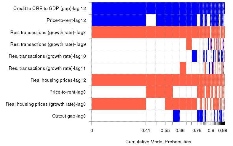
Figures 3 and 4 show which models actually perform better, for RRE and CRE respectively, scaled
by their posterior model probability (PMP). In the case of RRE, the best model (with 59% PMP) is
the one that includes the gap of residential transactions (lag 8), the level of real residential prices
(lag 12), the level and the gap of the ratio of loans to households to GDP (both with lag 12) while
the second model includes, in addition to the previous variables, the growth rate of loans to
households with lag 12 and has a PMP of 19%. In the case of CRE the best model has a PMP of
41% and includes the gap of credit to CRE to GDP (lag 12), price-to-rent (lag 12), the growth rate
of residential transactions (lag 8), the level and growth rate of real housing prices (lag 8 and lag 12,
respectively).
8
We use the BMS library in R (see Zeugner S., 2011).
9
The gap (i.e. the deviation of the variable from the medium-long term value) is calculated using a one-sided Hodrick-
Prescott filter, where the estimate at each point in time is based only on current and past information.
10
The information on credit and other banking data are from supervisory data. The sources of residential transactions
and property prices are Agenzia delle Entrate, Banca d’Italia, Istat and il Consulente Immobiliare, whereas value added
of construction sector and GDP are from ISTAT.
11
In the bad-loan-based model for RRE, the explanatory variables were the annual growth rate of residential
transactions, the annual growth rate of nominal residential prices, the ratio of loans to households to GDP, the gap of
gross value added of the construction sector and the gap of residential transactions; in the model for CRE, 10-year
government bond yields, the gap of gross value added of construction sector, price-to-income, the annual growth rate of
lending to CRE, the annual growth rate of residential transactions.
10Figure 3 - Best BMA models for RRE
Source: Based on Supervisory reports and Central Credit Register data.
Note: Blue corresponds to a positive coefficient, red to a negative coefficient and white to non-inclusion (coefficient
zero).
Figure 4 – Best BMA models for CRE
Source: Based on Supervisory reports and Central Credit Register data.
Note: Blue corresponds to a positive coefficient, red to a negative coefficient and white to non-inclusion (coefficient
zero).
In Figure 5, we report the out-of-sample forecasting exercise for RRE and CRE, the prediction of
the median level (solid dark red and blue lines, respectively) together with the 10th and 90th
percentile of their predictive density (dashed lines, red for RRE and blue for CRE). As we can see
the median predictions fit our new vulnerability indicators well; in particular they are able to
represent the decrease of vulnerability in the recent years.
11Figure 6 reports the projection results of the new early warning models in the fourth quarter of
2019: for RRE, the projections indicate a further slight decrease in the level of banking
vulnerability to an historical low level; for CRE, the projections indicate a stabilization of
vulnerability at pre-crisis levels.
Figure 5 – Out-of-sample prediction of the EWMs for RRE and CRE
(quarterly data; percentage points)
12 12
10 10
8 8
6 6
4 4
2 2
0 0
1990 1995 2000 2005 2010 2015
Vulnerability indicator RRE - Estimated New banks' vulnerability indicator related to RRE
Median - RRE 10 p - RRE
90 p - RRE Median - CRE
10 p - CRE 90 p - CRE
Vulnerability indicator CRE - Estimated New banks' vulnerability indicator related to CRE
Source: Based on Supervisory reports and Central Credit Register data.
Figure 6 – Forecasts of the new RRE and CRE models
(quarterly data; percentage points)
Source: Credit Register and Supervisory data
Note: Banks’ vulnerability is measured by the ratio of the flow of new NPLs in the last four quarters to the average of
the banks’ capital and reserves in the same period. The forecast relative to the fourth quarter of 2019 is graphically
represented by the median value (point) and the 10th and 90th percentile (bar). (2) The vulnerability indicators were
reconstructed backwards using econometric techniques for the period 1990-2005.
124. Robustness checks
In our analysis the selection of the optimal set of variables and the out-of-sample evaluation of the
BMA EWMs are made on the test period 2016q2-2018q3, where the new vulnerability indicator has
a persistently downward trend. As robustness checks for our methodology, we carried out the same
analysis by considering different training and test periods. The resulting best early warning
indicators could change at each different test period.
A first robustness check considers as a training set the period 1990q1–2007q4 and as a test set the
period 2009q1-2011q4, when banks’ vulnerabilities toward the real estate sector were building up.
The results,12 reported in Figure 7, show that the median predictions for RRE and CRE are able to
replicate reasonably well the increase in vulnerabilities during those years, especially for CRE.
A second check considers as a training set the period 1990q1–2011q1 and as a test set the period
2012q2-2014q3, when banks’ vulnerabilities were broadly stationary for the RRE sector and hump-
shaped for the CRE sector. The results,13 reported in Figure 8, show that the median predictions for
RRE correctly replicate the overall stable level of vulnerability of those years; while the median
predictions for CRE follow the non-linear trend of the indicator with a few quarters lag.
Figure 7 – Robustness check – test period 2009q1-2011q2
(quarterly data; percentage points)
14 14
12 12
10 10
8 8
6 6
4 4
2 2
Test set 2009q1- 2011q2
0 0
1990 1995 2000 2005 2010 2015
Vulnerability indicator RRE - Estimated New banks' vulnerability indicator related to RRE
Median - RRE 10th percentile - RRE
90th percentile - RRE Median - CRE
10th percentile - CRE 90th percentile - CRE
Vulnerability indicator CRE - Estimated New banks' vulnerability indicator related to CRE
Source: Credit Register and Supervisory data.
Note: The out-of-sample forecast is graphically represented by the median value (solid line) and the 10th and 90th
percentile (dashed lines).
12
In this case, the optimal sets of variables are: for RRE, price to rent (lag12), the gap of residential transactions (lag 8),
the growth rate of nominal housing prices (lag 12), the growth rate of residential transactions (lag 9), the growth rate of
disposable income (lag12); for CRE, price to rent (lag12), the growth rate of residential transactions (lag 8 and lag 9)
and the gap of credit to CRE to GDP (lag 12).
13
In this case, the optimal sets of variables are: for RRE, the gap of residential transactions (lag 8), real housing prices
(lag 10) and valued added construction to GDP (lag 10); for CRE, price to rent (lag12), the growth rate of residential
transactions (lag 10) and the growth rate of residential transactions (lag 8, lag 11 and lag 12).
13Figure 8 – Robustness check – test period 2012q2-2014q3
(quarterly data; percentage points)
18 18
16 16
14 14
12 12
10 10
8 8
6 6
4 4
2 2
0
Test set 2012q2- 2014q3 0
1990 1995 2000 2005 2010 2015
Vulnerability indicator RRE - Estimated New banks' vulnerability indicator related to RRE
Median - RRE 10th percentile - RRE
90th percentile - RRE Median - CRE
10th percentile - CRE 90th percentile - CRE
Vulnerability indicator CRE - Estimated New banks' vulnerability indicator related to CRE
Source: Credit Register and Supervisory data.
Note: The out-of-sample forecast is graphically represented by the median value (solid line) and the 10th and 90th
percentile (dashed lines).
5. Conclusions
In this work we provide an update of the analytical framework to assess financial stability risks
arising from the real estate sector in Italy. The enhancement concerns the definition of a new
banking vulnerability indicator, measured in terms of total non-performing loans and not in terms of
bad loans only as in the past, and its use in the estimation of the early warning models.
The decision to switch from a bad-loan-based indicator to a NPL-based banks’ vulnerability
indicator was motivated by both the greater attention to NPLs at national and international level,
and the fact that the increase of the flow of bad loans in recent years is not representative of higher
potential risks for the banking system but is rather related to past vulnerabilities and banks’ credit
management policies.
Two new NPL-based banking vulnerability indicators towards the real estate sector, for households
(i.e. the residential real estate sector, RRE) and for constructions and real estate agencies (i.e the
commercial real estate sector, CRE) respectively, are constructed for the period 1990-2006 using
some backdating techniques in order to recover sufficiently long time series for the estimation of
the early warning models. The new indicators, in line with the previous ones, highlight how in Italy
during the period 1990-2018 the risks for financial stability stemmed mainly from loans to
construction and real estate firms.
Two early warning models are estimated using the two new vulnerability indicators as dependent
variables. We consider the BMA methodology which allows us to identify the best set of early
warning indicators: for the RRE sector these are the residential transactions (both in terms of the
gap and growth rate), the ratio of loans to households to GDP (both in terms of levels and the gap),
the level of real residential prices and the annual growth rate of loans to households; for the CRE
14sector they are the ratio of loans to CRE to GDP (in terms of the gap), the price-to-rent ratio,
residential transactions (in terms of the growth rate), real residential prices (in terms of levels and
the growth rate) and the output gap. Overall, these indicators are consistent with those selected by
the previous models based on the bad-loans indicators.
Both early warning models exhibit good forecasting performances up to two years forward: the
median predictions fit well the new vulnerability indicators for RRE and CRE in the out-of-sample
period.
Overall, the model projections indicate that potential risks for banks stemming from the real estate
sector will remain moderate in the next few quarters. Based on projections for the fourth quarter of
2019, the new vulnerability indicator is expected to record another small decline, reaching a
historically low level for the RRE sector and to remain unchanged at pre-crisis levels for the CRE
sector.
15References
Agnello, L. and L. Schuknecht (2011), ‘Booms and busts in housing markets: Determinants and
implications’, Journal of Housing Economics 20(3): 171-190.
Alessi, L. and C. Detken (2011), ‘Quasi real time early warning indicators for costly asset price
boom/bust cycles: A role for global liquidity’. European Journal of Political Economy, 27(3): 520-
533.
Angelini, E., J. Henry, and M. Marcellino (2006), ‘Interpolation with a large information set’,
Journal of Economic Dynamics and Control, 30 (12): 2693-2724
Angelini, E. and Marcellino, M. (2007), ‘Econometric analyses with backdated data: Unified
Germany and the euro area’, ECB working paper n. 752/ 2007
Babecky, J., T. Havranek, J. Mateju, M. Rusnak, K. Smidkova and B. Vasicek (2012), ‘Banking,
debt and currency crises. Early warning indicators for developed countries’, ECB Working Paper
Series n. 1485.
Barrell, R, E.P. Davis, D. Karim and I. Liadze (2009), ‘Bank regulation, property prices and early
warning systems for banking crises in OECD countries’. NIESR Discussion Paper, n. 330.
Cerutti, E., J. Dagher, and G. Dell’Ariccia (2015), ‘Housing Finance and Real Estate Booms: A
Cross Country Perspective’, IMF Staff Discussion Note.
Chow, G.C. and A. Lin (1971), ‘Best linear Unbiased interpolation, Distribution and Extrapolation
of time series by related series’, Review of Economics and statistics, 53: 372-375.
Ciocchetta, F., W. Cornacchia, M. Loberto and R. Felici (2016), ‘Assessing financial stability risks
from the real estate market in Italy’, Occasional Paper n. 323 of the Bank of Italy.
Claessens S., M.Ayhan Kose and M.E. Terrones (2008), ‘What happens during recessions, crunches
and busts?’, IMF Working Paper n. 11/88.
Cornacchia W. and Pirovano, M. (2018), ‘A guide to early warning models for real estate related
banking crises’, in Recent trends in the real estate market and its analysis, Warsaw School of
Economics Press.
Diebold F.X. and J.A. Lopez (1996), ‘Forecast Evaluation and Combination’, in Handbook of
Statistics, Maddala GS, Rao CR eds.
Fernandez, C., E. Ley and M. Steel (2001a), ‘“Model Uncertainty in Cross-Country Growth
Regressions’, Journal of Applied Econometrics, 16: 563-576.
Fernandez, C., E. Ley and M. Steel (2001b), ‘Benchmark Priors for Bayesian Model Averaging’,
Journal of Econometrics 100: 381-427.
Ferrari S. and M. Pirovano (2014), ‘Evaluating early warning indicators for real estate related
risks’, National Bank of Belgium FSR.
16Ferrari S., M. Pirovano and W. Cornacchia (2015), dentifying early warning indicators for real
estate banking crises’, ESRB Occasional Paper n. 8.
Holopainen, M. and P. Sarlin (2015), ‘Toward robust early-warning models: A horse race,
ensembles and model uncertainty’, Bank of Finland, Research Paper 6/2015.
Geweke, J. and Whiteman, C. (2006), ‘Bayesian forecasting’, Handbook of Economic Forecasting,
1: 3–80, Elsevier.
Zeugner S. (2011), ‘Bayesian Model Averaging with BMS - for BMS version 0.3.0’, May 5th
(bms.zeugner.eu/tutorials/bms.pdf).
17You can also read