Supplement of HETEROFOR 1.0: a spatially explicit model for exploring the response of structurally complex forests to uncertain future conditions ...
←
→
Page content transcription
If your browser does not render page correctly, please read the page content below

Supplement of Geosci. Model Dev., 13, 905–935, 2020
https://doi.org/10.5194/gmd-13-905-2020-supplement
© Author(s) 2020. This work is distributed under
the Creative Commons Attribution 4.0 License.

Supplement of
HETEROFOR 1.0: a spatially explicit model for exploring the response
of structurally complex forests to uncertain future conditions – Part 1:
Carbon fluxes and tree dimensional growth
Mathieu Jonard et al.

Correspondence to: Mathieu Jonard (mathieu.jonard@uclouvain.be)

The copyright of individual parts of the supplement might differ from the CC BY 4.0 License.
HETEROFOR 1.0
                              User Manual

Mathieu Jonard, Frédéric André and Louis de Wergifosse

Faculty of Bioscience Engineering & Earth and Life Institute
Environmental sciences
Croix du Sud, 2 box L7.05.09 - 1348 Louvain-la-Neuve
mathieu.jonard@uclouvain.be
frederic.andre@uclouvain.be
louis.dewergifosse@uclouvain.be
Tel. +32 (0)10 47 25 48
Mobile +32 (0)499 39 28 91

                                      January 2020

                                             1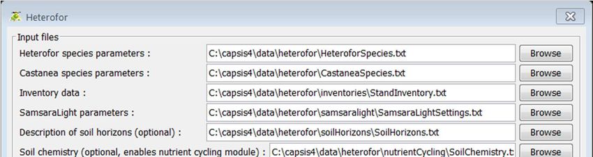
1. Table of content
            contents
             ontents

1. Table of contents ................................................................................................................................ 2
2. Introductory remarks.......................................................................................................................... 3
3. Installation of HETEROFOR under CAPSIS .......................................................................................... 3
4. Initialization of HETEROFOR ............................................................................................................... 4
5. Launching an evolution and planning silvicultural interventions ..................................................... 9
6. Launching a reconstruction .............................................................................................................. 11
7. Evaluation tools ................................................................................................................................ 13
   Evaluation based on soil water content data .................................................................................... 14
   Evaluation based on tree growth data .............................................................................................. 15
8. Model outputs (graphs and tables).................................................................................................. 17
9. Saving the project or the session ..................................................................................................... 21
10. Script mode ..................................................................................................................................... 22
11. References....................................................................................................................................... 22

                                                                           2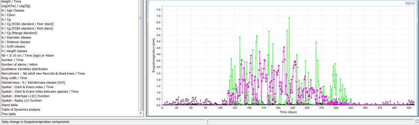
2. Introductory remarks

HETEROFOR is a tree-level model developed according to a spatially-explicit process-based approach
to explore the response of structurally-complex stands (uneven-aged, mixed) to changing
environmental conditions. Since 2012, HETEROFOR has been progressively elaborated through the
integration of various modules (light interception, phenology, water balance, photosynthesis and
respiration, carbon allocation, mineral nutrition and nutrient cycling) within CAPSIS, a collaborative
modelling platform dedicated to tree growth and stand dynamics (Dufour-Kowalski et al., 2012). A
general overview of the model functioning and a detailed description of the carbon-related processes
of HETEROFOR (photosynthesis, respiration, carbon allocation and tree dimensional growth) can be
found in Jonard et al. (2020). For the light interception, HETEROFOR is coupled to the SAMSARALIGHT
library first developed by Courbaud et al. (2003) and further adapted by Ligot et al. (2014) and André
et al. (in prep). The phenology and water balance module of HETEROFOR are presented in de
Wergifosse et al. (2020) while the mineral nutrition and nutrient cycling module must still be improved
and will be published later.

HETEROFOR was designed to be particularly suitable for the level II plots of ICP Forests. The processes
were described at a scale that facilitates the comparison between model predictions and observations.
Many data collected in these plots can be used to initialize and run the model or to calibrate and
evaluate it. HETEROFOR can also be seen as a tool for integrating forest monitoring data and
quantifying non-measured processes.

3. Installation of HETEROFOR under CAPSIS

The source code of CAPSIS and HETEROFOR is accessible to all the members of the CAPSIS co-
development community. Those who want to join this community are welcome but must contact
François      de       Coligny     (coligny@cirad.fr)      and      sign      the     CAPSIS     charter
(http://capsis.cirad.fr/capsis/charter). This charter grants access on all the models to the modellers of
the CAPSIS community. The modellers may distribute the CAPSIS platform with their own model but
not with the models of the others without their agreement. CAPSIS4 is a free software (LGPL licence)
which includes the kernel, the generic pilots, the extensions and the libraries. For HETEROFOR, we also
choose an LGPL license and decided to freely distribute it through an installer containing the CAPSIS4
kernel and the latest version (or any previous one) of HETEROFOR upon request from Mathieu Jonard
(mathieu.jonard@uclouvain.be). The source code for the modules published in Geoscientific Model
Development (Jonard et al., 2020; de Wergifosse et al., 2020) can be downloaded from
https://github.com/jonard76/HETEROFOR-1.0_LGPL_REVISED (DOI: 10.5281/zenodo.3591348).

The end-users can install CAPSIS from an installer containing only the HETEROFOR model while the
modellers who signed the CAPSIS charter can have access the complete version of CAPSIS with all the
models. Depending on your status (end-user vs modeller or developer), the instructions to install
CAPSIS are given on the CAPSIS website (http://capsis.cirad.fr/capsis/documentation).

Here is a brief explanation for installing CAPSIS under Windows using an installer. First, create/choose
a directory where the CAPSIS files will be stored. This can be called “Capsis”. Then, click on the CAPSIS
Installer (e.g., capsisHETEROFOR1.0 _setup.jar), follow the instructions and use the Capsis directory for
the installation. Open a command prompt and reach the Capsis directory using the “cd” command (cd..

                                                   3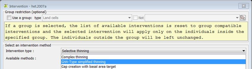
and cd directoryName). Allocate memory with the command “setmem 8000” and finally launch Capsis
from the Capsis directory using the command: “capsis -l en”.

4. Initialization of HETEROFOR

When CAPSIS is started, a first window appears and one can create a new project or open an existing
one. The user can also open an existing session containing several projects.

If “Create a new project” is chosen, a second window opens from which the HETEROFOR model can be
selected among the list of models available in CAPSIS. When an installer is used, only a subset of models
are available. To launch the model initialization, click on the Initialize button.

                                                   4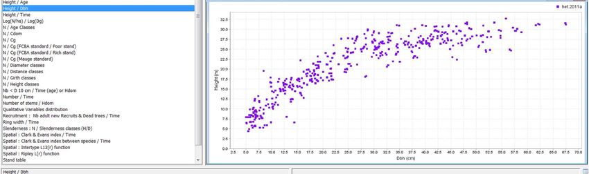
Initializing HETEROFOR requires a series of information provided by loading files and selecting model
options through the initial dialog.

When HETEROFOR is run with the default mode (i.e., no optional input file provided and no module
selection box checked), the vegetation period is defined based on the budburst and the leaf shedding
dates provided in the setting file of SAMSARALIGHT; no water balance is achieved; the gross primary
production (gpp) of each tree is calculated with a radiation use efficiency approach; the net primary
production (npp) is determined based on a fixed proportion of gpp and a distance-independent routine
is used to describe crown extension. The initial dialog allows the user to activate (i) the phenology
module either at the species level (default option for which all the trees of a same species have the
same phenology) or at the tree level (the trees of a same species have a phenology depending on their
size, see de Wergifosse et al. (2020)) (ii) the water balance module at the tree (fine resolution) or stand
level (the default option is the stand scale with a possibility to calculate transpiration at the tree level),
(iii) the coupling with CASTANEA for the photosynthesis calculation, (iv) the temperature-dependent
routine to determine maintenance respiration, (v) the soil heat transfer module (spatial resolution

                                                      5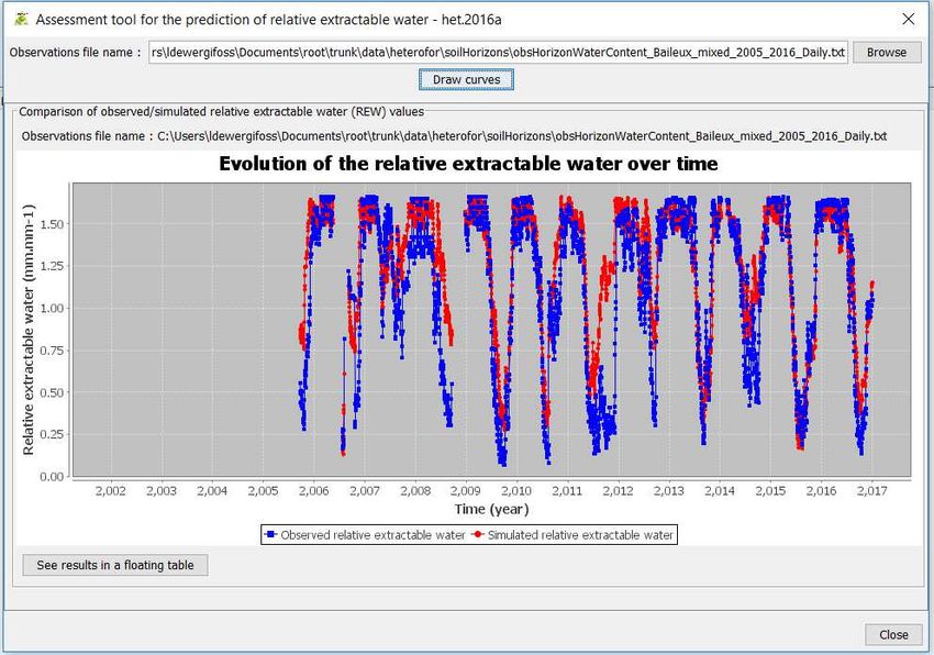
must be provided) and (vi) the distance-dependent approach to describe crown extension. The user
can also define the time step at which the radiative budget must be performed and whether the
detailed approach must be used. The model can account for the nutrient limitation of tree growth with
the possibility to select an approach particularly adapted to nitrogen. These nutritional aspects being
still under testing, we recommend not using this option for the moment. For the photosynthesis
estimated with CATANEA, the model can either consider a fixed atmospheric CO2 concentration or load
a file describing its temporal change according to various IPCC scenarios (yearly time step). Several
approaches were tested to estimate the height growth. We recommend to select the “Baileux” option
which has been described in Jonard et al. (2020). Finally, one can choose to activate the mortality
routine and select the branch and trunk diameter under which the wood is not harvested and left in
the forest (which has implications for the nutrient budget).

Besides this selection of options, three parameter/setting files must be provided since two CAPSIS
libraries (SAMSARALIGHT for light interception and CASTANEA for photosynthesis) are used in addition
to HETEROFOR. For HETEROFOR and CASTENEA, the parameters are mostly species specific; they are
defined in Jonard et al. (2020) and de Wergifosse et al. (2020) regarding HETEROFOR and in Dufrêne
et al. (2005) for CASTANEA. The setting parameters needed to initialize SAMSARALIGHT as well as the
description of the functioning of this library are presented on the CAPSIS website at
http://capsis.cirad.fr/capsis/help_en/samsaralight.

Then, the user must provide an inventory file containing the relative position (x, y, z) and the main
dimensions of each tree: girth at breast height (gbh in cm), height (h in m), height of maximum crown
extension (hlce in m), height to crown base (hcb in m) and crown radii in the four cardinal directions
(cr in m). This file also specifies the site name, the starting date, the cell size for the radiation transfer
module, the maximum leaf area index for the whole ecosystem, the tree compartments (leaves,
branches, stem, roots) and litter nutrient concentrations, the latitude, longitude and slope of the site
(in degrees), the clockwise angle of the slope bottom from the North (site aspect, in degrees) and the
clockwise angle between North and the x axis (in degrees). When data on fruit litterfall are available,
a file providing the amount of fruit litterfall per year and per tree species can be loaded and used to
adapt the allometric equations predicting fruit production at the individual level.

When the water balance module is activated, two additional files must be loaded: a file describing soil
horizon properties and another one for the meteorology. For each horizon, the following properties
are provided: upper and lower horizon limits (m), total (m³ total stone .m-³ total soil) and sampling (m³
stone in Kopecky .m-³ Kopecky) coarse fraction, bulk density (kg.m-3), sand, silt and clay contents (g.g-
1
 ), organic carbon (mg.g-1), mean, wilting point and saturated water content (m-3.m-3), soil solution pH,
log pCO2 (with pCO2 in atm), fine root proportion (%) and tortuosity factor (m.m-1). The meteorological
data are read by a loader and stored in hourly meteo line objects containing the date split in four fields
(year, month, day, hour) and seven meteorological variables: radiation (W.m-²), air temperature (°C),
soil surface temperature (°C), rainfall (l.m-2 or mm), relative humidity (% or hPa / 100 hPa), wind speed
(m.s-1) and wind direction (degrees).

Finally, the soil chemistry input file must be provided when the nutritional limitation is considered.
This file contains 6 parts:

    -   a list with all the chemical elements, their charge and atomic mass,
    -   the element concentrations in the soil solution for each soil horizon (K, Ca, Mg, Na, Nam, Al,
        Mn(2), Fe(3), Cl, Nnit, S(6), P, Si, Cit, C(4) in mg.l-1),
    -   the exchangeable cation concentrations for each cation exchanger (Xo, Xm, Xs) and soil horizon
        (e.g. HXo, KXo, CaXo2, MgXo2, NaXo, NamH4Xo, AlXo3, MnXo2, FeXo3, HXm, KXm, CaXm2,

                                                      6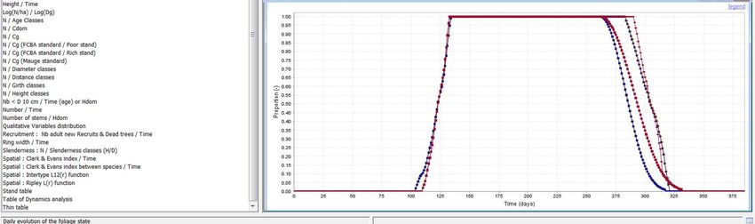
MgXm2, NaXm, NamH4Xm, AlXm3, MnXm2, FeXm3, HXs, KXs, CaXs2, MgXs2, NaXs, NamH4Xs,
    AlXs3, MnXs2, FeXs3 in cmole.kg-1),
-   the exchangeable anion concentrations for each anion exchanger (Ya) and soil horizon (e.g.
    YaCl, YaNnitO3, Ya2SO4, YaH2PO4, YaH3SiO4, Ya3Cit, YaHCO3, YaOH in cmole.kg-1),
-   the mineral properties: mineral type (e.g., quartz, K-feldspar, K-mica, illite, albite, anorthite,
    chlorite(14A), Vrm, kaolinite, variscite, Ca-Montmorillonite, manganite, Fe(OH)3(a)),
    concentration in mole/kg, weathering type (1 for equilibrium and 2 for kinetics), target
    saturation index as log(IAP/Ks) with IAP: ion activity product and Ks: solubility product of the
    mineral (all dimensionless), reaction type (d for dissolution, p for precipitation and b for both),
    kinetics parameters depending on the formula mentioned in the PHREEQC database,
-   the atmospheric deposition (in kg.ha-1.year-1).

After selecting the desired options and specifying the paths to the input files, the initialization can
be launched by pressing on the “Ok” button. The model creates then a new project with only the
initial step corresponding to the state of the forest stand at the starting date mentioned in the
inventory file. The stand can be visualize in 2D by selecting the “scene viewer” tab (choose
Heterofor viewer) on the left panel. This viewer shows the tree crowns and the relative light
transmitted to the ground cells. To obtain a 3D representation of the stand, the user must choose
the 3D viewer in the lower right panel and select the trees with the mouse (right click).

                                                7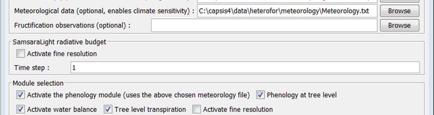
8
5. Launching an evolution and planning silvicultural interventions

Right-click on the initial step and select “Evolution” in the drop-down menu to launch a simulation.

A window appears and allows the user to specify the length of the simulation and to load a file listing
the trees to be thinned and their last year of presence in the stand.

The simulation can take several minutes depending on its length. When the evolution is finished, the
project is composed of as many steps as years in the evolution. Each step correponds to a year and
contains the state of the stand at the end of this year (after the vegetation period).

The thinning file is optional and, alternatively, thinning can also be achieved by right clicking on the
step after which the thinning must be done and selecting “Intervention” in the drop-down menu. In
the window that appeared, choose “Selective thinning” in the intervention type. You will then have
access to all the routines created in CAPSIS to achieve a thinning as far as they are compatible with
HETEROFOR. The user is referred to the documentation of CAPSIS for a detailed description of these
thinning routines called interveners (http://capsis.cirad.fr/capsis/documentation/interventions).

                                                   9
10
6. Launching a reconstruction

HETEROFOR was adapted to allow the user to run it in reverse mode starting from the known
increments in girth and height to reconstruct individual tree growth using exactly the same parameters
and equations as in the normal mode. To achieve a reconstruction, an inventory file with tree
measurements must be loaded to create the initial step (see sect. 5.). The reconstruction tools can be
launched by right-clicking on the initial step and select “Tool box” in the drop-down menu. Then, the
user must choose the reconstruction tool (Heterofor Reconstruction of Observed Growth) and provide
an inventory file with tree measurements achieved one or several years later as well as the thinning
file. Based on these files, HETEROFOR calculates the mean girth and height increments for each tree
and use the model equations to reconstruct each step. Do not forget to click on the “Launch
estimation” button.

                                                 11
After a while, a graph showing the PAR use efficicency as a function of the light competition index
will appear. The project corresponding to the growth reconstruction will appear after clicking on the
initial step.
127. Evaluation tools
Different evaluation tools can be used in HETEROFOR to compare the model predictions with the
observations. A visual comparison is proposed by default but a txt file and a table with the
corresponding predictions and observations can be created and opened, respectively. The visualisation
tools can be access with a right-click on the step for which or until which observations are available
and by selecting “Tool box” (Ctrl+B).
Different toolboxes are available but only three are evaluation tools: the assessment tool for the
prediction of relative extractable water (REW), the assessment tool for the prediction of water content
and the HETEROFOR prediction assessment tool which is dedicated to the evaluation of tree
dimensional growth.
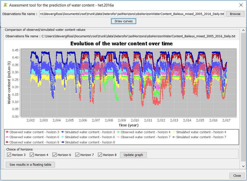
13Evaluation based on soil water content data
Both evaluation tools for REW and water content predictions require the same observational file. This
file is a table providing the water content (in m³.m-3) per soil horizon for each day or hour. The date is
indicated based on three or four fields: Year, Month, Day, Hour.
For the REW evaluation tool, the resulting graph displays the temporal evolution of the predicted and
observed REW. The REW is calculated according to de Wergifosse et al. (in review) by considering only
the horizons for which water content data are available. Missing data do not prevent the evaluation
tool to run but it will generate discontinuities in the graph.
The second tool displays the temporal variability of predicted and observed water content per soil
horizon. For better legibility, it is recommended to select one horizon at a time.
14For both evaluation tools, the data can be visualized in a table by clicking on “See results in a floating
table”.
Evaluation based on tree growth data
The tool to assess tree growth requires an inventory file similar to the one used for the initialization
but for a later date in order to calculate the increments in girth, height and crown dimensions. The
user must select the step for which a repeated inventory is available and load the corresponding file.
A large amount of graphs is displayed after a short calculation time. The data corresponding to these
graphs can be obtained by right-clicking on them and select “extract in a table”.
Three types of evaluation graphs are proposed. First, bar charts compare mean predictions and
observations for the various tree species (see previous figure). Such graphs are available for the girth
increment (cm.yr-1), basal area increment (cm².yr-1), height increment (m.yr-1), crown base height
increment (m.yr-1), largest crown extension increment (m.yr-1) and the quadratic crown radius
increment. Second, scatter plots compare predicted vs observed size-growth relationships. Two types
of relationships are available: the height increment (m.yr-1) as a function of initial height (m) and the
basal area increment (cm².yr-1) as a function of initial girth (cm).
15Third, scatter plots comparing observations with predictions enable to assess the quality of the
predictions (with reference to the 1:1 line) and detect some eventual biases. For some graphs, trees
are grouped per girth class while, for others, the observations and predictions correspond to individual
trees. Such graphs are available for the girth increment (cm.yr-1), the basal area increment (cm².yr-1),
the height increment (m.yr-1), the crown base height increment (m.yr-1), the largest crown extension
increment (m.yr-1) and the crown radius increments in the four cardinal directions (with and without
log transformation).
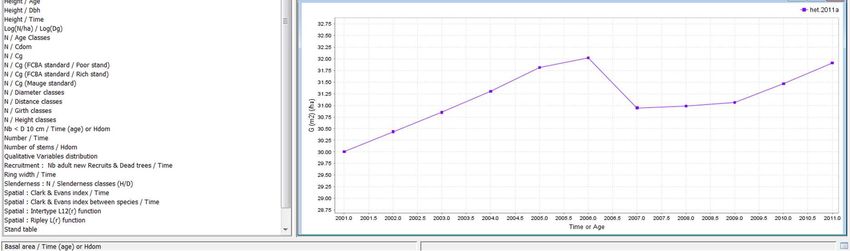
168. Model outputs (graphs and tables)
The user has at his disposal a whole series of graphs created for all individual-based models in CAPSIS.
These graphs are listed on the left panel when the “Chart” tab is selected. To create a graph for a given
simulation, select the corresponding project in the upper right panel and double-click on the graph
name in the list. It will then appear in the lower right panel. For example, a graph shows the temporal
trend in basal area or its evolution with dominant height. The layout of this graph can be modified by
right-clicking on it and selecting “Configure”. For the basal area graphs, one can choose the unit for
the basal area (in m² or in m².ha-1) or the variable of the X axis (Time or Dominant height).
Graphs displaying temporal trends can also be obtained for other variables: geometric mean or
dominant girth/dbh, girth/dbh of selected trees (right-click on the graph and choose “Configure” to
select the trees of interest), LAI and dominant height. Some graphs are present in the list but do not
appear correctly when selected. This happens for the graphs showing an evolution with tree age
because tree age is not considered in HETEROFOR. Other graphs are showing relationships between
tree dimensions (e.g., height vs dbh) or between stand variables (e.g., log N vs log mean dbh). One can
also create tables with stand characteristics or histograms showing the distribution of trees per size
class.
Besides these default graphs available for all individual-based models of CAPSIS, some charts are
specific to HETEROFOR. Among them, a graph shows the daily evolution in the foliage state for each
tree species, if the phenology module was activated at initialization. The state of the foliage is
characterized by two variables:
- ladProp: the proportion [0-1] of leaf with reference to the maximum leaf amount when the
full leaf development is reached,
- greenProp: the proportion of green leaves with reference to maximum leaf amount.
One can zoom on the graph with the left-click. The data used to create the graph can be obtained by
right-clicking on the graph and selecting “open in a floating table”.
1718
19
Similar graphs show the daily change in rainfall partitioning, evapotranspiration components, deep
drainage and relative extractable water.

In addition to these graphs, the state variables of HETEOFOR can be visualized in tables and exported
in txt files. To generate an export, right-click on the final step of a project and select “Export”. You will
have access to a list of exports through the window here below and have to specify where the txt file
must be stored.

                                                     20
Many variables can be exported and concerns the foliage state (see above), the phenological dates
corresponding to the main phenological events, the tree characteristics, the hourly soil temperature,
the water fluxes and contents at yearly, monthly, daily or hourly time step, the nutrient fluxes and
stocks (in the trees an in the soil) and the soil chemistry.
9. Saving the project or the session
The project can be save by selecting it and then choose “save” or “save as” in drop-down menu
under “Project”.
Similarly, the session containing all the projects can be saved.
2110.
10. Script mode
CAPSIS is generally used in interactive mode which allows the users to work in a graphical environment
with menus and dialogs as described above. Alternatively, the script mode can also be very useful to
execute long and repetitive simulations. The results of these simulations are saved in files that can be
analysed later in Capsis or with other analysis or statistical tools. The script mode is also very
interesting to call CAPSIS from another software (such as R) in order to, for example, perform a
calibration of the model parameters. All the information needed to create a script is available at
http://capsis.cirad.fr/capsis/documentation/script_mode
11.
11. References
Courbaud, B., de Coligny, F., Cordonnier, T. 2003. Simulating radiation distribution in a heterogeneous
Norway spruce forest on a slope. Agricultural and Forest Meteorology, 116, 1-18.
de Wergifosse, L., André, F., Beudez, N., de Coligny, F., Goosse, H., Jonard, F., Ponette, Q., Titeux,
H., Vincke, C., and Jonard, M. 2020. HETEROFOR 1.0: a spatially explicit model for exploring the
response of structurally complex forests to uncertain future conditions. II. Phenology and water cycle,
Geosci. Model Dev. Discuss.
Dufour-Kowalski, S., Courbaud, B., Dreyfus, P., Meredieu, C., de Coligny, F. 2012. Capsis: an open
software framework and community for forest growth modelling. Annals of Forest Science, 69, 221–
233.
Dufrêne, E., Davi, H., François, C., Le Maire, G., Le Dantec, V., Granier, A. 2005. Modelling carbon and
water cycles in a beech forest: Part I: Model description and uncertainty analysis on modelled NEE.
Ecological Modelling, 185, 407-436.
Jonard, M., André, F., de Coligny, F., de Wergifosse, L., Beudez, N., Davi, H., Ligot, G., Ponette, Q., and
Vincke, C. 2020. HETEROFOR 1.0: a spatially explicit model for exploring the response of structurally
complex forests to uncertain future conditions. I. Carbon fluxes and tree dimensional growth, Geosci.
Model Dev. Discuss.
Ligot, G., Balandier, P., Courbaud, B., Jonard, M., Kneeshaw, D. 2014. Managing understory light to
maintain a mixture of species with different shade tolerance. Forest Ecology and Management, 327,
189-200.
22You can also read