Learning How to Autonomously Race a Car: a Predictive Control Approach
←
→
Page content transcription
If your browser does not render page correctly, please read the page content below
Learning How to Autonomously Race a Car:
                                                                        a Predictive Control Approach
                                                                                          Ugo Rosolia and Francesco Borrelli

                                           Abstract—In this paper we present a Learning Model Pre-                 Contouring Control (MPCC) was presented in [16]. In MPCC
                                        dictive Controller (LMPC) for autonomous racing. We model                  the controller objective is a trade-off between the progress
                                        the autonomous racing problem as a minimum time iterative                  along the track and the contouring error. First, an high level
                                        control task, where an iteration corresponds to a lap. The system
                                        trajectory and input sequence of each lap are stored and used              MPC computes the optimal racing trajectory. Afterward, a low
                                        to systematically update the controller for the next lap. In the           level controller is used to track the optimal racing line. This
                                        proposed approach the race time does not increase at each                  strategy is extended in [17] to design a racing controller which
arXiv:1901.08184v3 [cs.SY] 4 Oct 2019

                                        iteration. The first contribution of the paper is to propose a             guarantees recursive constraint satisfaction. Also in [18] the
                                        local LMPC which reduces the computational burden associated               control problem is divided in two steps. First, a reference
                                        with existing LMPC strategies. In particular, we show how to
                                        construct a local safe set and approximation to the value function,        trajectory is computed using the method proposed in [19].
                                        using a subset of the stored data. The second contribution is to           Afterwards, an iterative learning control (ILC) approach is
                                        present a system identification strategy for the autonomous racing         used for tracking. The authors showed the effectiveness of
                                        iterative control task. We use data from previous iterations and           the proposed approach by experimental testing on a full size
                                        the vehicle’s kinematic equations of motion to build an affine             vehicle. We proposed to reformulate the autonomous racing
                                        time-varying prediction model. The effectiveness of the proposed
                                        strategy is demonstrated by experimental results on the Berkeley           problem as an iterative control task. The controller is not based
                                        Autonomous Race Car (BARC) platform.                                       on a precomputed racing line and it learns from experience
                                                                                                                   a trajectory which minimizes the lap time. In particular,
                                                                                                                   the closed-loop trajectories at each lap are stored used to
                                                                I. I NTRODUCTION                                   systematically update the controller for the next lap. This paper
                                           Autonomous driving is an active research field. Over the                builds on [20]–[22] and has two main contributions.
                                        past decades several techniques have been proposed for differ-                The first contribution is to propose a local LMPC strat-
                                        ent driving scenarios [1]–[9]. Depending on the control task               egy where the terminal cost and constraint are updated at
                                        (i.e. highway driving, urban driving, emergency maneuvers)                 each time step. In particular at each time t, we exploit the
                                        the behavior of the vehicle can be modelled with linear or                 planned trajectory at time t − 1 to construct a local terminal
                                        nonlinear equations of motions [10], [11]. When the nonlin-                cost and constraint. Conversely to our previous works [20]–
                                        earities of the vehicle are excited the control task is inevitably         [22], the terminal cost and constraint are computed using a
                                        more challenging. In this work we are interested in designing              subset of the stored data, therefore the proposed local LMPC
                                        a controller for autonomous racing which can operate the                   enables the reduction of computational burden associated with
                                        vehicle in the nonlinear regime, close to the limit of the                 existing LMPC strategies. The effectiveness of the proposed
                                        vehicle’s handling capability. We formulate the autonomous                 approach is demonstrated on the Berkeley Autonomous Race
                                        racing problem as an iterative control task, where at each                 Car (BARC)1 platform. We show that the proposed controller
                                        iteration the controller drives the vehicle around the track               is able to improve the lap time, until it converges to a steady
                                        trying to minimize the lap time.                                           state behavior. Finally, we analyze the lateral acceleration
                                           Recently several approaches have been proposed for au-                  acting on the closed-loop system and we confirm that the
                                        tonomous racing. In [12] the authors reformulated the au-                  controller learns to drive the vehicle at the limit of its handling
                                        tonomous racing control task as a non-convex optimization                  capability.
                                        problem and then proposed a linearization strategy to compute                 The second contribution of this work is to propose a system
                                        an approximate solution. The authors in [13] proposed a                    identification strategy tailored to the autonomous racing appli-
                                        Nonlinear Model Predictive Control (NMPC) strategy which                   cation. We propose to exploit both the kinematic equations
                                        exploits a Pacejka tire model identified form experimental                 of motion and data from previous iterations to identify an
                                        data. The NMPC is implemented on an experimental set-                      Affine Time Varying (ATV) prediction model used for control.
                                        up using an exact Hessian SQP-type optimization algorithm.                 In particular, we use a local linear regressor to learn the
                                        NMPC strategies for autonomous racing are tested also in                   relationships between the inputs and the vehicle’s velocities.
                                        [14], where the authors compared two control methodologies                 Furthermore, we linearize the kinematic equations of motion
                                        based on different parametrizations of the vehicle’s model.                to approximate the evolution of the vehicle’s position as a
                                        In [15] the authors compared two approaches, the first one                 function of the velocities. Conversely to our previous works
                                        based on a tracking MPC and the second one based on a MPC                  [20], [21], this strategy allow us to reformulate the LMPC as
                                        formulated in a space dependent frame. A Model Predictive                  a Quadratic Program (QP) which can be solved efficiently.
                                          U. Rosolia and F. Borrelli are with the Department of Mechanical Engi-
                                                                                                                      This paper is organized as follows: in Section II we intro-
                                        neering, University of California at Berkeley , Berkeley, CA 94701, USA
                                        {ugo.rosolia, fborrelli}@berkeley.edu                                        1A   video of the experiment can be found at https://youtu.be/ZBFJWtIbtMo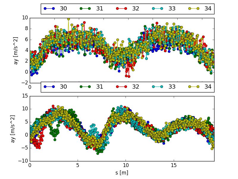
duce the problem formulation. Section III illustrates the LMPC                                                III. C ONTROLLER D ESIGN
design. In particular, it shows how to construct local safe                           In this section, we first show how to use historical data to
sets and value function approximations using a subset of the                        construct a terminal constraint set and terminal cost function.
collected data. Section IV illustrates the system identification                    Afterwards, we exploit these quantities to design the controller.
strategy used in the experiments. Finally, in Section V we
present the experimental results on the Berkeley Autonomous
Race Car (BARC) platform. Section VIII provides final re-                           A. Stored Data
marks.                                                                                As stated in the introduction, we define one iteration as a
                                                                                    successful lap around the race track and we store the closed-
                                                                                    loop trajectories. In particular, at the jth iteration we define
                       II. P ROBLEM F ORMULATION
                                                                                    the vectors
   Consider the following state and input vectors                                                        uj = [uj0 , . . . , ujT j ]
                                                                                                                                                 (4)
                                     >         >                                                     xj = [xj0 , . . . , xjT j ],
        x = vx , vy , wz , eψ , s, ey    and u = δ, a ,
                                                                                    which collect the evolution of closed-loop system and associ-
where wz , vx , vy , are the vehicle’s yaw rate, longitudinal and                   ated input sequence. In the above definitions, T j denotes the
lateral velocities. The position of the vehicle is represented in                   time at which the closed-loop system reached the terminal set,
the curvilinear reference frame [23], where s is the distance                       i.e. xT j ∈ XF .
travelled along the centerline of the track. The states eψ and
ey are the heading angle and lateral distance error between the
vehicle and the centerline of the track, as shown in Figure 1.                      B. Local Convex Safe Set
Finally, δ and a are the steering and acceleration commands.                           In this section, we define the local convex safe set. Dif-
The vehicle is described by the dynamic bicycle model                               ferently from our previous works [20]–[22], this quantity
                                                                                    is constructed using a subset of the stored data points. In
                                  xt+1 = f (xt , ut ),                        (1)   particular, the local convex safe set around x is defined as
                                                                                    the convex hull of the K-nearest neighbors to x.
where f (·, ·) is derived from kinematics and balancing the
                                                                                       First, for the jth trajectory we define the set of time indices
forces acting on the tires [10]. A detailed expression can be
                                                                                    [tj,∗          j,∗
                                                                                      1 , . . . , tK ] associated with the K-nearest neighbors to the
found in [10, Chapter 2]. Note that in the curvilinear reference
                                                                                    point x,
frame state and input constraints are convex, i.e.
                                                                                                                             K
                 xt ∈ X = {x ∈ Rn : Fx x ≤ bx },                                    [tj,∗          j,∗
                                                                                                                                   ||xjti − x||2D
                                                                                                                             X
                                                                                      1 , . . . , tK ] = argmin
                                        d                                                                     t1 ,...,tK
                 ut ∈ U = {u ∈ R : Fu u ≤ bu }, ∀t ≥ 0.                                                                      i=1
                                                                                                                      s.t.   ti 6= tk , ∀i 6= k
                                                                                                                  ti ∈ {0, . . . , T j }, ∀i ∈ {1, . . . , K}.
                                                         s                                                                                                 (5)
           distance travelled along the path                 ey                     In the above definition ||y||2D = y > D> Dy for the user-defined
                                                                                    matrix D, which may be chosen to take into account the
                                                                                    relative scaling or relevance of different variables. We chose
                                                                                    D = diag(0, 0, 0, 0, 1, 0) to select the K-nearest neighbors
path’s origin
                                                                                    with respect to the curvilinear abscissa s, which represents a
Fig. 1. Representation of the vehicle’s position in the curvilinear reference       proxy for the distance between two stored data points of the
frame.                                                                              same lap. Furthermore, as the vehicle moves forward on the
   The goal of the controller is to drive the system from the                       track, at each lap the stored data are ordered with respect to the
starting point xS to the terminal set XF . More formally, the                       travelled distance s and the computation of (5) is simplified.
controller aims to solve the following minimum time optimal                         The K-nearest neighbors to x from the lth to the jth iteration
control problem                                                                     are collected in the following matrix

                       T −1                                                                   Dlj (x) = [xltl,∗ , . . . , xltl,∗ , . . . , xjtj,∗ , . . . , xjtj,∗ ],
                       X                                                                                          1              K             1               K
       min                    1
  T,u0 ,...,uT −1                                                                   which is used to define the local convex safe set around x
                       t=0
                s.t.   xt+1 = f (xt , ut ),         ∀t = [0, . . . , T − 1]           CLjl (x) = {x̄ ∈ Rn : ∃λ ∈RK(j−l+1) ,
                       xt ∈ X , ut ∈ U,             ∀t = [0, . . . , T ]                                         λ ≥ 0, 1λ = 1, Dlj (x)λ = x̄}.
                                                                                                                                                (6)
                       xT = XF , x0 = xS ,
                                                                              (2)   Notice that the above local convex safe set CLjl (x) represents
where for a track of length L the terminal set                                      the convex hull of the K-nearest neighbors to x from the lth
                                                                                    to jth iteration.
                XF = {x ∈ Rn : [0 0 0 0 1 0]x = s ≥ L}                        (3)      Finally, we define the matrix

represents the states beyond the finish line.                                           Slj (x) = [xltl,∗ +1 , . . . , xltl,∗ +1 , . . . , xjtj,∗ +1 , . . . , xjtj,∗ +1 ]
                                                                                                          1                  K                 1                   K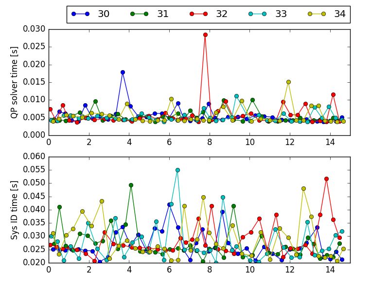
which collects the evolution of the states stored in the columns is used to compute the following vector
of the matrix Dlj (x). The above matrix Slj (x) will be used in (
Section III-D to construct the local convex safe set at each j xj−1
N If t = 0
zt = , (10)
time step. Slj (zt−1
j
)λj,∗
t−1 Otherwise
which at time t defines the local convex safe set LS jl (ztj )
C. Local Convex Q-function
and local Q-function Qjl (x, ztj ) in (8). The above vector ztj
In this section, we exploit the stored data to construct an represents a candidate terminal state for the planned trajectory
approximation to the cost-to-go over the local convex safe set of the LMPC at time t. First, we initialize the candidate
CLjl (x) around x. In particular, we define the local convex terminal state z0j using the (j − 1)th trajectory. Afterwards,
Q-function around x as the convex combination of the cost we update the vector ztj as the convex combination of the
associated with the stored trajectories, columns of the matrix Slj (ztj ) from Section III-B. Notice that
Qjl (x̄, x) = min Jjl (x)λ if the systems is linear or if a linearized system approximates
λ (7) the nonlinear dynamics over the local convex safe set, then
s.t λ ≥ 0, 1λ = 1, Dlj (x)λ = x̄, there exists a feasible input which drives the system from
xj,∗
t+N |t = Dt
j−1 j
(zt )λj,∗
t
j
to zt+1 = Slj−1 (ztj )λj,∗
t .
where λ ∈ Rk(j−l) , 1 is a row vector of ones and the row
Finally, we apply to the system (1) the first element of the
vector
optimizer vector,
Jjl (x) = [Jtll,∗ →T l (xltl,∗ ), . . . , Jtll,∗ →T l (xltl,∗ ), . . . , ujt = uj,∗
1 1 M M t|t . (11)
Jtjj,∗ →T j (xjtj,∗ ), . . . , Jtjj,∗ →T j (xjtj,∗ )], The finite time optimal control problem (8) is repeated at time
1 1 M M
t + 1, based on the new state xt+1|t+1 = xjt+1 .
collects the cost-to-go associated with the K-nearest neighbors
j j
to x from the lth the jth iteration. The cost-to-go Jt→T j (xt ) =
j j IV. S YSTEM I DENTIFICATION S TRATEGY
T − t represents the time to drive the vehicle from xt to the
finish line along the jth trajectory. We underline that the cost- In this section, we illustrate the system identification strat-
to-go is computed after completion of the jth iteration. egy used to build an Affine Time Varying (ATV) model which
approximates the vehicle dynamics. First, we introduce the
D. Local LMPC Design kinematic equations of motion which describe the evolution
The local convex safe set and the local convex Q-function of the vehicle’s position as a function of the velocities.
are used to design the controller. At each time t of the jth Afterwards, we present the strategy used to approximate the
iteration the controller solves the following finite time optimal dynamic equations of motion, which model the evolution of
control problem the vehicle’s velocities as a function of the input commands.
Finally, we describe the ATV model, which is computed online
LMPC,j
Jt→t+N (xjt , ztj ) = linearizing the kinematic equations of motion and evaluating
t+NX−1 the approximate dynamic equations of motion along the shifted
j j−1 j j
min
j j
h(xk|t ) + Jl (zt )λt (8a) optimal solution to the LMPC.
Ut ,λt
k=t
s.t. xjt|t = xjt , (8b) A. Kinematic Model
λjt ≥ 0, 1λjt = 1, Dlj−1 (ztj )λjt = xjt+N |t (8c) As mentioned in Section II, the position of the vehicle is
xjk+1|t = Ajk|t xjk|t + Bk|t
j
ujk|t + Ck|t
j
, (8d) expressed in the Frenet reference frame [23]. In particular, we
j j describe the position of the vehicle in terms of lateral distance
xk|t ∈ X , uk|t ∈ U, (8e) ey from the centerline of the road and distance s traveled
∀k = t, · · · , t + N − 1, along a predefined path (Fig. 1). The state eψ represents the
difference between the vehicle’s heading angle and the angle
where Ujt = [ujt|t , . . . , ujt+N −1|t ] ∈ Rd×N , λjt ∈ R(j−l+1)K of the tangent vector to the path at the curvilinear abscissa s.
and the stage cost in (8a) The rate of change of the vehicle’s position in the curvili-
nar reference frame is described by the following kinematic
(
1 If x ∈ / XF
h(x) = . relationships
0 Else
vx cos(eψ ) − vy sin(eψ )
In the above finite time optimal control problem equations ėψ = wz − κ(s)
1 − κ(s)ey
(8b), (8d) and (8e) represent the dynamic update, state and
input constraints. Finally, (8c) enforces xjt+N |t into the local vx cos(eψ ) − vy sin(eψ )
ṡ =
convex safe set defined in Section III-B. The optimal solution 1 − κ(s)ey
to (8) at time t of the jth iteration ėy = vx sin(eψ ) + vy cos(eψ ),
λtj,∗ , [xj,∗ j,∗ j,∗ j,∗ j,∗
t|t , . . . , xt+N |t ] and Ut = [ut|t , . . . , ut+N −1|t ] where κ(s) is the curvature of the centerline of the track at the
(9) curvilinear abscissa s [23]. The above equations can be Eulerdiscretized to approximate the vehicle’s motion as a function where ||y||Q = y > Q> Qy and the matrix Q is user defined.
of the vehicle’s velocities For the stored data from iteration l to iteration j, the set Ilj (x)
eψk+1 = feψ (xk ) = eψk collects the indices associated with the P -nearest neighbors
! to the state x. Finally, the user-defined matrix Q takes into
vxk cos(eψk ) − vyk sin(eψk ) account the relative scaling of different variables.
+ dt wzk − κ(sk )
1 − κ(sk )eyk Notice that the optimizer in (13) can be used to approximate
the evolution of vehicle’s velocities,
!
vxk cos(eψk ) − vyk sin(eψk )
sk+1 = fs (xk ) = sk + dt
1 − κ(sk )eyk
vxk+1
vx
Γ1:3 (x)
vx k
vyk+1 = Γv1:3
! y
(x) vyk
ėy = fey (xk ) = eyk + dt vxk sin(eψk ) + vyk cos(eψk ) , wzk+1 wz
Γ1:3 (x) wzk
vx vx
(12) Γ4 (x) 0 Γ5 (x)
v a v
where dt is the discretization time. The above equations will + 0 Γ4y (x) k + Γ5y (x) ,
wz δk wz
be linearized to compute an ATV prediction model. It is 0 Γ4 (x) Γ5 (x)
interesting to notice that equations (12) are independent of (14)
the vehicle’s physical parameters, because these are derived where for l = {vx , vy , wz } the scalar Γli (x) denotes the ith
from kinematic relationships between velocities and position. element of the vector Γl (x) and Γl1:3 (x) ∈ R3 is a row vector
collecting the first three elements of Γl (x) in (13).
B. Dynamic Model
The dynamic equations of motion, which describe the evo- C. Affine Time Varying Model
lution of the vehicle’s velocities, may be computed balancing
the forces acting on the tires [10]. Therefore, the dynamic In this section we describe the strategy used to build an ATV
equations depend on physical parameters associated with the model, which is then used for control. At time t of the jth iter-
vehicle, tires and asphalt. These parameters may be estimated ation we define the candidate solution x̄jt = [x̄jt|t , . . . , x̄jt+N |t ]
through a system identification campaign. However, the non- to Problem (8) using the optimal solution at time t−1 from (9),
linear dynamic equations of motion should be linearized in (
order to obtain an ATV model which allows us to reformulate j xj,∗
k|t−1 If k ∈ {t, . . . , t + N − 1}
the LMPC as a QP. Instead of identifying the parameters of a x̄k|t = j .
zt If k = t + N
nonlinear model and then linearize it, we propose to directly
learn a linear model around x using a local linear regressor. Finally at each time t of iteration j, the above candidate
We introduce the Epanechnikov kernel function [24] solution is used to build the following ATV model
(
3
(1 − u2 ), for |u| < 1
K(u) = 4 , xjk+1|t = Ajk|t xjk|t + Bk|t
j
ujk|t + Ck|t
j
, (15)
0, else
which is used to compute a local linear model around x for where xjk|t = [vxj k|t , vyj k|t , wyj k|t , ejψk|t , sjk|t , ejyk|t ] and the ma-
the longitudinal and lateral dynamics. In particular, for l =
trices Ajk|t , Bk|t
j j
and Ck|t are obtained linearizing (12) around
{vx , vy , wz } we compute the following regressor vector
x̄jk|t and evaluating (14) at x̄jk|t ,
||x − xjk ||2Q j,l
!
X
l
Γ (x) = argmin K yk (Γ), (13)
Γv1:3 (x̄jk|t ) 0 0 0
Γ h x vx j
{k,j}∈I(x)
vy j Γ4 (x̄k|t ) 0
Γ1:3 (x̄k|t ) 0 0 0
v
where the hyperparameter h ∈ R+ is the bandwidth, the row 0 Γ4y (x̄jk|t )
wz j
Γ1:3 (x̄ ) 0 0 0
vector Γ ∈ R5 , Γw j
= 0 4 (x̄k|t )
k|t z
Ajk|t
j
= (∇ f (x)| j )> , Bk|t
x eψ
ykj,vx (Γ) ajk , x̄k|t 0 0
= ||vxj k+1 − Γ[vxj k , vyj k , wzjk , 1]T ||
(∇x fs (x)|x̄j )>
0 0
j,v
yk y (Γ) = ||vyj k+1 − Γ[vxj k , vyj k , wzjk , δkj , 1]T || k|t
0 0
(∇x fey (x)|x̄j )>
ykj,wz (Γ) = ||wzjk+1 − Γ[vxj k , vyj k , wzjk , δkj , 1]T ||, k|t
(16)
and
and Ilj (x) is the set of indices
Γv5x (x̄jk|t )
P
Ilj (x) xjkii ||2Q
X
= argmin ||x − v
Γ5y (x̄jk|t )
{k1 ,j1 },...,{kP ,jP }
i=1
Γw (x̄jk|t )
z
5
s.t. Ck = f (x̄j ) − (∇ f (x)| j )> x̄j .
(17)
ki 6= kn , ∀ji = jn ey k|t x ey x̄k|t k|t
fs (x̄j ) − (∇x fs (x)| j )> x̄j
ki ∈ {1, 2, . . .}, ∀i ∈ {1, . . . , P } k|t x̄k|t k|t
ji ∈ {l, . . . , j}, ∀i ∈ {1, . . . , P }, feψ (x̄jk|t ) − (∇x feψ (x)|x̄j )> x̄jk|t
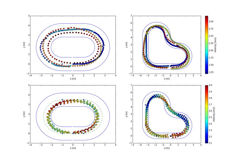
k|tV. R ESULTS We tested the controller on an oval-shaped and L-shaped
The proposed control strategy has been implemented on tracks on which the vehicle runs in the counter-clockwise
a 1/10-scale open source vehicle platform called Berkeley direction. Figure 2 shows that the lap time decreases until
Autonomous Race Car2 (BARC). The vehicle is equipped with convergence is reached after 29 laps. Furthermore, Figure 4
a set of sensors, actuators and two on-board CPUs to perform shows the evolution of the closed-loop trajectory on the X-
low-level control of the actuators as well as communication Y plane and the velocity profile which is color coded. In the
with a laptop, on which the high-level control is implemented. first row we reported the path following trajectory used to
The CPUs are an Arduino Nano for low-level control of the initialize the LMPC and the closed-loop trajectories at laps 7
actuators and an Odroid XU4 for WiFi communication with and 15. We notice that the controller deviates from the initial
the i7 MSI GT72 laptop. The actuators are an electrical motor feasible trajectory (reported in blue as the vehicle speed is
and a servo for the steering. The control architecture has been 1.2m/s) in order to explore the state space and to drive the
implemented in the Robot Operating System (ROS) frame- vehicle at higher speeds, until it converges to a steady-state
work, using Python and OSQP [25]. The code is available behavior. The steady-state trajectories from lap 30 to 34 are
online3 . reported in the bottom row of Figure 4. Notice that the color
bar representing the velocity profile changed from the first to
second row as the vehicle runs at higher speed at the end of the
learning process. We underline that the controller understands
the benefit of breaking right before entering the curve and of
accelerating when exiting. This behavior is optimal in racing
as shown in [26].
Fig. 2. Lap time of the LMPC on the oval-shaped and L-shaped tracks.
We initialize the algorithm performing two laps of path
following at constant speed. Each jth iteration collects the
data of two consecutive laps. Therefore, the local safe set and
local Q-function are defined also beyond the finish line. This
Fig. 3. Recorded lateral acceleration of the vehicle running on the oval-shaped
strategy allows us to implement the LMPC for the repetitive track (top row) and L-shaped track (bottom row).
autonomous racing control task, as shown in [20]. At each jth
lap, we use the LMPC (8) and (11) to drive the vehicle from Figure 3 shows the raw acceleration measurements from the
the starting line to the finish line and we use the closed-loop IMU. We confirm that controller is able to operate the vehicle
data to update the controller for the next lap. The parameters at the limit of its handling capability, reaching a maximum
which define the controller are reported in Table I. We also lateral acceleration close to 1g 4 .
added a small input rate cost in order to guarantee a unique Furthermore, Figure 5 shows the data points used to design
solution to the QP associated with the LMPC. the LMPC. Recall from Table I that at the jth lap the LMPC
policy is synthesized using the trajectories from lap l = j−2 to
TABLE I lap j −1. Therefore, as the controller drives faster on the track,
PARAMETERS USED IN THE CONTROLLER DESIGN . less data points are needed to design the LMPC. Moreover, in
l j−2 Figure 6 we reported the computational time. It is interesting to
K 20 notice that on average the finite time optimal control problem
T diag(0, 0, 0, 0, 1, 0) (8) is solved in less then 10ms, whereas it took 90ms to
Q diag(0.1, 1, 1, 0, 0, 0)
P 80 solve the finite time optimal control problem associated with
h 10 [20]. We underline that both strategies have been tested with
N 12 a prediction horizon of N = 12 and a sampling time of 10Hz.
2A video of the experiment can be found at https://youtu.be/ZBFJWtIbtMo 4 The maximum allowed lateral acceleration is computed assuming that the
3 The code is available on the BARC GitHub repository in the “devel-ugo” aerodynamic effects are negligible and the that lateral force acting on the
branch (github.com/MPC-Berkeley/barc) vehicle is F = µmg for the friction coefficient µ = 1.Fig. 4. The first row in the above figure shows the closed-loop trajectory used to initialize the LMPC and the closed-loop trajectories after few laps of
learning. The second row shows the steady state trajectories at which the LMPC has converged. Notice that the scale of the color bar changes from the first
to the second row, as the vehicle runs at higher speed after the learning process has converged.
of the N − 1 linear models which define the ATV model from
(15). Indeed, at time t Equations (16)-(17) may be evaluated
independently and in parallel for each predicted time k.
Fig. 5. Data points used in the LMPC design at each lap.
This shows the advantage of using the local convex safe set
in (6), instead of the polynomial approximation to the safe
set used in [20], [21]. For more details on the polynomial Fig. 6. In the first and the second row is shown the computational cost asso-
ciated with the FTOCP and the system identification procedure, respectively.
approximation to the safe set we refer to [21]. Finally, we
notice that it would be possible to parallelize the computationVI. C ONCLUSIONS [16] A. Liniger, A. Domahidi, and M. Morari, “Optimization-based au-
tonomous racing of 1: 43 scale rc cars,” Optimal Control Applications
We presented a Learning Model Predictive Controller and Methods, vol. 36, no. 5, pp. 628–647, 2015.
(LMPC) for autonomous racing. The proposed control frame- [17] A. Liniger and J. Lygeros, “Real-time control for autonomous racing
work uses historical data to construct safe sets and approxima- based on viability theory,” IEEE Transactions on Control Systems
Technology, no. 99, pp. 1–15, 2017.
tions to the value function. These quantities are systematically [18] N. R. Kapania and J. C. Gerdes, “Path tracking of highly dynamic au-
updated when a lap is completed, as a result the LMPC learns tonomous vehicle trajectories via iterative learning control,” in American
from experience to safely drive the vehicle at the limit of Control Conference (ACC), 2015. IEEE, 2015.
[19] P. A. Theodosis and J. C. Gerdes, “Generating a racing line for an au-
handling. We demonstrated the effectiveness of the proposed tonomous racecar using professional driving techniques,” in ASME 2011
strategy on the Berkeley Autonomous Race Car (BARC) Dynamic Systems and Control Conference and Bath/ASME Symposium
platform. Experimental results show that the controller learns on Fluid Power and Motion Control. American Society of Mechanical
Engineers, 2011, pp. 853–860.
to drive the vehicle aggressively, in order to minimize the [20] M. Brunner, U. Rosolia, J. Gonzales, and F. Borrelli, “Repetitive learning
lap time. In particular, the closed-loop system converged to a model predictive control: An autonomous racing example,” in 2017 IEEE
steady-state trajectory which cuts curves and reaches a lateral 56th Annual Conference on Decision and Control (CDC), Dec 2017, pp.
2545–2550.
acceleration close to 1g. [21] U. Rosolia, A. Carvalho, and F. Borrelli, “Autonomous racing using
learning model predictive control,” in 2017 American Control Confer-
R EFERENCES ence (ACC), May 2017, pp. 5115–5120.
[1] E. J. Rossetter and J. C. Gerdes, “Lyapunov based performance guaran- [22] U. Rosolia and F. Borrelli, “Learning model predictive control for
tees for the potential field lane-keeping assistance system,” Journal of iterative tasks: A computationally efficient approach for linear system,”
dynamic systems, measurement, and control, vol. 128, no. 3, pp. 510– IFAC-PapersOnLine, vol. 50, no. 1, pp. 3142–3147, 2017.
522, 2006. [23] A. Micaelli and C. Samson, “Trajectory tracking for unicycle-type and
[2] Y. Gao, A. Gray, J. V. Frasch, T. Lin, E. Tseng, J. K. Hedrick, two-steering-wheels mobile robots,” Ph.D. dissertation, INRIA, 1993.
and F. Borrelli, “Spatial predictive control for agile semi-autonomous [24] V. A. Epanechnikov, “Non-parametric estimation of a multivariate prob-
ground vehicles,” in 11th International Symposium on Advanced Vehicle ability density,” Theory of Probability & Its Applications, vol. 14, no. 1,
Control, 2012. pp. 153–158, 1969.
[3] Y. Kuwata, J. Teo, G. Fiore, S. Karaman, E. Frazzoli, and J. P. How, [25] B. Stellato, G. Banjac, P. Goulart, A. Bemporad, and S. Boyd, “Osqp:
“Real-time motion planning with applications to autonomous urban An operator splitting solver for quadratic programs,” in 2018 UKACC
driving,” IEEE Transactions on Control Systems Technology, vol. 17, 12th International Conference on Control (CONTROL). IEEE, 2018,
no. 5, pp. 1105–1118, 2009. pp. 339–339.
[4] J. V. Frasch, A. Gray, M. Zanon, H. J. Ferreau, S. Sager, F. Borrelli, [26] P. A. Theodosis and J. C. Gerdes, “Nonlinear optimization of a racing
and M. Diehl, “An auto-generated nonlinear mpc algorithm for real-time line for an autonomous racecar using professional driving techniques,”
obstacle avoidance of ground vehicles,” in Control Conference (ECC), in ASME 2012 5th Annual Dynamic Systems and Control Conference.
2013 European. IEEE, 2013, pp. 4136–4141. American Society of Mechanical Engineers, 2012, pp. 235–241.
[5] M. Campbell, M. Egerstedt, J. P. How, and R. M. Murray, “Autonomous
driving in urban environments: approaches, lessons and challenges,”
Philosophical Transactions of the Royal Society of London A: Math-
ematical, Physical and Engineering Sciences, vol. 368, no. 1928, pp.
4649–4672, 2010.
[6] D. González, J. Pérez, V. Milanés, and F. Nashashibi, “A review of
motion planning techniques for automated vehicles,” IEEE Transactions
on Intelligent Transportation Systems, vol. 17, no. 4, pp. 1135–1145,
2016.
[7] C. Katrakazas, M. Quddus, W.-H. Chen, and L. Deka, “Real-time motion
planning methods for autonomous on-road driving: State-of-the-art and
future research directions,” Transportation Research Part C: Emerging
Technologies, vol. 60, pp. 416–442, 2015.
[8] B. Paden, M. Čáp, S. Z. Yong, D. Yershov, and E. Frazzoli, “A survey of
motion planning and control techniques for self-driving urban vehicles,”
IEEE Transactions on Intelligent Vehicles, vol. 1, no. 1, pp. 33–55, 2016.
[9] G. Williams, P. Drews, B. Goldfain, J. M. Rehg, and E. A. Theodorou,
“Aggressive driving with model predictive path integral control,” in
Robotics and Automation (ICRA), 2016 IEEE International Conference
on. IEEE, 2016, pp. 1433–1440.
[10] R. Rajamani, Vehicle dynamics and control. Springer Science &
Business Media, 2011.
[11] A. Alleyne, “A comparison of alternative intervention strategies for
unintended roadway departure (urd) control,” Vehicle System Dynamics,
vol. 27, no. 3, pp. 157–186, 1997.
[12] B. Alrifaee and J. Maczijewski, “Real-time trajectory optimization for
autonomous vehicle racing using sequential linearization,” in 2018 IEEE
Intelligent Vehicles Symposium (IV). IEEE, 2018, pp. 476–483.
[13] R. Verschueren, S. De Bruyne, M. Zanon, J. V. Frasch, and M. Diehl,
“Towards time-optimal race car driving using nonlinear mpc in real-
time,” in 53rd IEEE conference on decision and control. IEEE, 2014,
pp. 2505–2510.
[14] R. Verschueren, M. Zanon, R. Quirynen, and M. Diehl, “Time-optimal
race car driving using an online exact hessian based nonlinear mpc
algorithm,” in 2016 European Control Conference (ECC). IEEE, 2016,
pp. 141–147.
[15] R. Verschueren, S. De Bruyne, M. Zanon, J. V. Frasch, and M. Diehl,
“Towards time-optimal race car driving using nonlinear mpc in real-
time,” in 53rd IEEE Conference on Decision and Control. IEEE, 2014,
pp. 2505–2510.You can also read


