THE IMPACT OF A MASS RAPID TRANSIT SYSTEM ON NEIGHBORHOOD HOUSING PRICES: AN APPLICATION OF DIFFERENCE-IN- DIFFERENCE AND SPATIAL ECONOMETRICS ...
←
→
Page content transcription
If your browser does not render page correctly, please read the page content below
www.degruyter.com/view/j/remav

        THE IMPACT OF A MASS RAPID TRANSIT
         SYSTEM ON NEIGHBORHOOD HOUSING
      PRICES: AN APPLICATION OF DIFFERENCE-IN-
       DIFFERENCE AND SPATIAL ECONOMETRICS
 Lee Chun-Chang
 National Pingtung University, Taiwan
 e-mail: lcc@mail.nptu.edu.tw

 Liang Chi-Ming
 National Taipei University of Business, Taiwan
 e-mail: lcc@mail.nptu.edu.tw

 Hong Hui-Chuan
 National Pingtung University, Taiwan
 e-mail: lcc@mail.nptu.edu.tw
                                                    Abstract
 This study discusses the impact of the mass rapid transit (MRT) system’s construction and operation
 on neighborhood housing prices. Estimations were conducted by considering the spatial dependence
 of housing prices and using a difference-in-difference (DD) method that incorporated the spatial lag
 model and spatial error model. The empirical results indicated that the coefficient of the interaction
 variable of the MRT’s range of influence and commencement time of construction was -0.079, reaching
 the 10% significance level. Hence, when MRT construction began, housing prices in the experimental
 group decreased by 7.9% as compared to the control group. A possible reason for these findings is that
 the “dark age” of urban traffic, air pollution, and noise brought about by MRT construction negatively
 affected housing prices. With regard to MRT operations, the coefficient of the interaction variable of
 the MRT’s influence range and service commencement time did not reach the level of significance,
 indicating that housing prices within the MRT’s influence range were not significantly affected when
 the MRT’s service began. This might be due to the fact that the psychological expectations of the
 increase in housing prices had already been realized during the planning, announcement, and
 construction phases.

 Key words: housing prices; mass rapid transit, geographic information system, difference-in-difference, spatial
 error model, spatial lag model.

 JEL Classification: C21, O18, P25.

 Citation: Chun-Chang, L., Chi-Ming, L. & Hui-Chuan, H. (2020). The impact of mass rapid transit
 system on neighborhood housing prices: an application of difference-in-difference and spatial
 econometrics. Real Estate Management and Valuation, 28(1), 28-40.

 DOI: https://doi.org/10.2478/remav-2020-0003

 1. Introduction
 Mass rapid transit (MRT) systems are an important means of transportation in Taiwan. For instance,
 the Taipei Metro, the MRT system with the longest operating history in Taiwan, has solved the issue
 of traffic congestion in the metropolitan area. The Taipei Metro launched its services in 1996 and has

 28            REAL ESTATE MANAGEMENT AND VALUATION, eISSN: 2300-5289

vol. 28, no. 1, 2020
www.degruyter.com/view/j/remav
been operating for over 20 years. The metro consists of five lines, namely: the Wenhu, Tamsui-Xinyi,
Songshan-Xindian, Zhonghe-Xinlu, and Bannan lines, and 117 stations. The MRT system has partially
alleviated traffic issues, increased commuting convenience, and promoted the rise of neighborhood
housing prices.
Studies by Dziauddin et al. (2013) and Ryan (2005) indicated an increase in housing prices near the
metro and light rail stations. Bowes and Ihlanfeldt (2001) also maintained that metro stations can
cause an increase in neighborhood housing prices. McMillen and McDonald (2004) studied the effect
of a MRT line from downtown Chicago to Midway Airport on neighboring housing prices before and
after the line opened. The empirical results showed that housing prices were already affected in the
1980s and early 1990s, prior to the opening of the line. This indicates that housing prices are affected
by the anticipated construction of a MRT. Between 1986 to 1999, housing prices within 1.5 miles of the
line increased by US$216 million. Yiu and Wong (2005) analyzed the impact of the MRT system on
neighborhood housing prices using a hedonic price model and found that the construction of
transport had a significant positive influence on neighborhood housing prices. The increased
accessibility of MRT reduces commute time, making it an incentive to purchase housing near MRT
stations. Agostini, Palmucci (2008) and Ge et al. (2012) suggested that announcements regarding the
commencement and completion of transport system construction, as well as its launching, had a
different effect on housing prices. Bowes and Ihlanfeldt (2001) and Boymal et al. (2013) analyzed the
influence of transportation facilities on neighborhood housing prices and found that MRT stations had
a significant positive effect on neighborhood housing prices. Wen, Gui, et al. (2018) suggested that the
ordinary least squares (OLS) regression model can only estimate the mean implicit prices of housing
characteristics and may ignore the various effects of mass transit systems on different housing prices.
On the other hand, quantile regression can explain how changes in the implicit prices of housing
attributes are affected by changes in housing prices. They used housing prices in Hangzhou, China,
and adopted the OLS model and quantile regression model approaches to measure the capitalization
effects of mass transit systems on housing prices. The empirical results showed that the housing prices
of units located within 2 km of an MRT station were 2.1% to 6.1% higher than the prices of those
located outside the 2 km range. The estimated coefficient increased from 0.023 in the 0.15 quantile to
0.086 in the 0.95 quantile. Therefore, mass transit systems will increase the capitalization effect of
transport accessibility.
Billings (2011) and Dubé et al. (2013) investigated the impact of transportation facilities on
neighborhood prices before and after policy announcements, at the beginning of construction, and at
the beginning of service. This study suggested that MRT affects housing prices during both the
construction and operation phases. Both phases were examined in order to explore the differences in
the effects of MRT on neighborhood housing prices at different stages of operation.
According to Tobler’s (1970) first law of geography, all objects are inter-related and their
correlation increases with proximity. The housing-housing relationship can be affected by
neighborhood housing prices. Dubin (1998) indicated that housing prices can be predicted by
establishing a hedonic regression based on housing characteristics and employing the ordinary least
squares (OLS) method as a statistical tool. However, this method ignores the issue of the spatial
correlation between neighborhood housing prices. A study by Chen and Haynes (2015) confirmed the
presence of spatial dependence in housing prices. The failure to solve the issue of spatial dependence
can cause bias in coefficient estimations. Diao, Leonard and Sing (2017) utilized Singapore’s new
Circle Line (CCL) as a natural experiment and used the spatial differences-in-differences approach to
examine the effects of network distance on non-landed housing prices. The empirical results showed
that the opening of the CCL will increase housing prices in the experimental zone (within a 600-meter
range of CCL stations) by 8.6%, approximately S$380.12 million, relative to the control zone after
controlling for heterogeneities in housing attributes, nearby facilities and spatial and temporal fixed
effects. The results of estimations are rendered more accurate by using the shortest network distance
measure for assessment, while the Euclidean distance measure will decrease the estimated coefficient.
There were anticipation effects one year prior to the opening of the CCL line, but these effects
gradually diminished with time. Housing prices were mostly affected during Phase 2 and Phase 3 of
the opening of the MRT line. Spatial dependence was observed in housing in the experimental and
control zones, and such a dependence will cause errors in estimations if neglected. Kopczewska and
Lewandowska (2018) utilized spatial modelling to measure the spatial econometrics and location
REAL ESTATE MANAGEMENT AND VALUATION, eISSN: 2300-5289 29
vol. 28, no. 1, 2020www.degruyter.com/view/j/remav
effects of office rental rates. Their empirical results indicate that geographical factors increased office
rental rates by about 50%, and the rates increased by about 0.7 pounds per square foot for every 100
feet closer to an MRT station, while rental rates in the city center increased by 20 pounds per square
foot in the same manner. Trojanek and Gluszak (2018) used the ordinary least squares approach
(OLS), spatial autoregressive model (SAR), spatial error model (SEM) and spatial general model
(SGM) integrated with the differences-in-differences (DID) approach to investigate the effect of MRT
lines on housing prices. They discovered that the housing prices were already affected prior to the
opening of the MRT. This study considered the possible effect of neighborhood housing prices on
housing prices. Housing prices near an area with high housing prices are likely to be high, whereas
housing prices near an area with low housing prices are likely to be low. In addition to the difference-
in-difference (DD) method, this study also integrated spatial econometrics. A spatial econometric
model was applied to explore the influence of neighborhood housing prices on housing prices and to
reduce the potential bias of the traditional regression model.
The Xinyi line of the Taipei Metro was examined in this study. The construction of the Xinyi line
began in 2005, and it was put into service on November 24, 2013, making it the second Taipei Metro
line to operate in the east-west direction. This study employed the DD method. The start of the
construction was set as the dividing time point and metro operation was designated as the influencing
event to examine the influence of metro construction and operation on neighborhood housing prices.
Furthermore, spatial dependence between housing prices, which is ignored in the traditional
regression model, was considered. Thus, in addition to the DD method, a spatial econometric model
was used in the analyses. The objectives of this study were to explore (1) the changes in housing prices
within the MRT range of influence after the beginning of metro construction and operation, as well as
the differences with respect to the influence of MRT construction time and operation time on housing
prices within the specified influence range, and (2) the spatial autocorrelation between neighborhood
housing prices and the influence of neighborhood housing prices on housing prices.
2. Methods
2.1. Empirical Model Establishment
The DD method is applied to evaluate differences in influence before and after an event or policy
implementation. Therefore, the affected group was set as the experimental group and the non-affected
group was set as the control group. The experimental and control groups were further divided into
the control group before the policy/event, experimental group before the policy/event, control group
after the policy/event, and experimental group after the policy/event, and differences between the
groups were analyzed. In this study, two policies were evaluated. The beginning of metro
construction and beginning of metro operation were set as the events that influenced neighborhood
housing prices; changes before and after these events were measured. Areas within the metro
influence range were included in the experimental group, and areas outside this range were included
in the control group. A DD model was established and used as the basis for the spatial lag model and
spatial error model used in the analyses.
First, the independent variables related to housing characteristics that could affect housing prices
included the age of the building ( AGE ), the age of the building squared ( AGE 2 ), the number of
rooms ( ROOM ), the number of living rooms ( LIVROOM ), number of bathrooms ( BATH ),
housing type ( TYPE ), location on the first floor ( FLOOR1 ), and location on the fourth floor (
FLOOR4 ). Variables in the DD method included metro influence time ( TIMEt ), metro influence
range ( MRTi ), and metro influence range metro influence time ( MRTi TIMEt ). The DD model
was established as shown in Equation (1):
ln Pit 1 2 AGEit 3 AGEit 4 ROOM it 5 LIVROOM it 6 BATH it 7TYPEit
2
(1)
8 FLOOR1it 9 FLOOR4 it 10TIMEt 11 MRTi TIMEt MRTi eit
where 1 is the intercept; 2 ~ 9 are coefficients of structural characteristics of housing; and 10 ,
11 , and are coefficients of metro influence time, metro influence range, and the interaction of
30 REAL ESTATE MANAGEMENT AND VALUATION, eISSN: 2300-5289
vol. 28, no. 1, 2020www.degruyter.com/view/j/remav
metro influence time and metro influence range, respectively. eit is the normally distributed error
term. The equation was evaluated using OLS.
Second, a spatial lag model was established based on the DD model, as shown in equation (2):
ln Pit 1 W ln Pit 2 AGEit 3 AGEit 4 ROOM it 5 LIVROOMit 6 BATH it
2
(2)
7TYPEit 8 FLOOR1it 9 FLOOR4 it 10TIMEt 11 MRTi TIMEt MRTi it
where 1 is the intercept; 2 ~ 9 are coefficients of the structural characteristics of housing; and
10 , 11 , and are coefficients of metro influence time, metro influence range, and the interaction of
metro influence time and metro influence range, respectively. W ln Pit is the explained variable
multiplied by the spatial weights matrix W . is the spatial lag coefficient. eit is the error term.
0 indicated spatial autocorrelation between neighborhood housing prices.
Third, a spatial error model was established based on the DD model, as shown in Equation (3):
ln Pit 1 2 AGEit 3 AGEit 4 ROOM it 5 LIVROOM it 6 BATH it 7TYPEit
2
(3)
8 FLOOR1it 9 FLOOR4 it 10TIMEt 11 MRTi TIMEt MRTi it
where 1 is the intercept; 2 ~ 9 are coefficients of structural characteristics of housing; and 10 , 11 ,
and are coefficients of metro influence time, metro influence range, and the interaction of metro
influence time and metro influence range, respectively. it is the error term. The error term after
correction was as shown in Equation (4):
it W it , ~ N 0 , 2
(4)
is the spatial error coefficient. 0 indicated spatial correlation in the spatial error regression
model due to confounding factors (ANSELIN 1988).
2.2. Establishment and Explanation of Variables
The dependent variable in this study was the logarithm of the total real estate transaction price.
Independent variables in this study included the age of the building ( AGEit ), the age of the building
2
squared ( AGE it ), the number of rooms ( ROOMit ), number of living rooms ( LIVROOMit ), the
number of bathrooms ( BATH it ), location on the first floor ( FLOOR1it ), location on the fourth floor (
FLOOR4it ), and housing type ( TYPE it ). Coefficients of the number of rooms ( ROOMit ), number
of living rooms ( LIVROOMit ), and number of bathrooms ( BATH it ) were expected to be positive
values.
The variable related to the beginning of metro construction and operation ( TIMEt ) was
established as follows. With regard to the beginning of construction, the transaction data sample was
collected from January 2004 to December 2006, and the year 2005 was set as the time point when
construction of the Xinyi line began. Data prior to and after the beginning of construction was coded
as 0 and 1, respectively. With regard to the commencement of operation, the data sample was
collected from January 2011 to December 2014. November 2013 was set as the time point when the
Xinyi line was introduced into service. Data prior to and after the beginning of operation was coded as
0 and 1, respectively.
With regard to the metro station influence range, Gibbons and Machin (2005) evaluated housing
prices within 1.25 miles from stations in London. Cervero and Duncan (2002) explored the impact of
the California Santa Clara light rail and commuter rail on neighborhood housing prices by setting 1/4
mile (approximately 400 meters) as the influence range. In a study by Armstrong and Rodriguez
(2006), housing prices within 1/2 mile from a station were 10.1% higher than those outside this range.
Dewees (1976) set 1/3 mile (approximately 500 meters) as the range of stations’ influence on housing
REAL ESTATE MANAGEMENT AND VALUATION, eISSN: 2300-5289 31
vol. 28, no. 1, 2020www.degruyter.com/view/j/remav
prices. Taiwanese scholars Feng, Tseng and Wang (1994) included areas within 500 meters from each
MRT station in the influence range, which was further subdivided for the metropolitan zone (0-100
meters), marginal zone (100-300 meters), and suburban zone (300-500 meters). According to the MRT
line planning principles published on the website of the Department of Rapid Transit Systems, Taipei
City Government, distance between stations should be maintained within 800-1000 meters in city
center areas and 1000-2000 meters in suburban areas as part of the road network plan,. Moreover, in
order to ensure MRT accessibility, distance between stations should not exceed 2400 meters. This
study considered walking distance and the fact that MRT stations’ influence ranges should not
overlap. Therefore, a 500-meter distance from an MRT station was established as the main research
range using GIS. Housing units within the 500-meter influence range were included in the
experimental group, and housing units outside the influence range were included in the control
group. With regard to the metro station influence range ( MRTi ) variable, data within the 500-meter
influence range of MRT stations was coded as 1 and data outside this range was coded as 0.
The interaction variable of the beginning of metro construction and operation and metro station
influence range (TIMEt MRTi ) referred to the location within the influence range after the
beginning of metro construction and operation. Due to environmental pollution caused by the
produced dust and the “dark age” of traffic caused by traffic inconvenience, the coefficient related to
the location within the influence range after the beginning of construction was predicted to be
negative. The coefficient related to the location within the influence range after the beginning of
operation was predicted to be positive. Coefficients related to this variable were DD coefficients (Table
1).
Table 1
Definition of variables
Expected
Variable Definition
Sign
ln Pit Logarithm of the total price of housing (incl. objects) transaction.
Based on the difference between the date of building construction
AGEit -
completion and the date of transaction, measured in years.
Based on the difference between the date of building construction
2
AGE it completion and the date of transaction and squared, measured in +
years.
ROOMit Number of rooms in the building. +
LIVROOMit Number of living rooms in the building. +
BATH it Number of bathrooms in the building. +
Location on the first floor was set as a dummy variable, with 1
indicating the first floor and 0 indicating other floors. The first floor
FLOOR1it +
can be used for shops and has a commercial value. Therefore,
housing prices were predicted to be high.
Location on the fourth floor was set as a dummy variable, with 1
indicating the fourth floor and 0 indicating other floors. In
FLOOR4it Mandarin, the pronunciation of “four” resembles that of “death” -
and, therefore, there is a bias towards the fourth floor. Thus, the
prices of housing on the fourth floor were predicted to be low.
Housing types included apartment buildings, multistoried
residential buildings, and mansions. The housing type was set as a
TYPEit +
dummy variable, with 1 indicating multistoried buildings and
mansions and 0 indicating apartment buildings.
With regard to the beginning of construction, the transaction data
sample was collected from January 2004 to December 2006, and the
TIMEt year 2005 was set as the time point when construction of the Xinyi +
line began. Data prior to and after the beginning of construction was
coded as 0 and 1, respectively. With regard to the beginning of
32 REAL ESTATE MANAGEMENT AND VALUATION, eISSN: 2300-5289
vol. 28, no. 1, 2020www.degruyter.com/view/j/remav
operation, the data sample was collected from January 2011 to
December 2014. November 2013 was set as the time point when the
Xinyi line was introduced into service. Data prior to and after the
beginning of operation was coded as 0 and 1, respectively.
This study considered walking distance and the fact that MRT
stations’ influence ranges should not overlap. Therefore, a 500-meter
distance from an MRT station was established as the main research
MRTi +
range. Housing units within the 500-meter influence range were
coded as 1 and housing units outside the influence range were
coded as 0.
Due to environmental pollution caused by the produced dust and
the “dark age” of traffic caused by traffic inconvenience, the
coefficient related to the location within the influence range after the
MRTi TIMEt beginning of construction was predicted to be negative. The +/-
coefficient related to the location within the influence range after the
commencement of operation was predicted to be positive.
Coefficients related to this variable were DD coefficients.
Source: own study.
3. Data Collection and Sample Statistics
3.1. Data Source Explanation
Housing transaction data in this study was obtained from the reports on Taiwan real estate
transactions published by the Department of Land Administration of the Ministry of the Interior and
GigaHouse. Taipei City was set as the research range, with the main research areas including the
Da’An District, Zhongzheng District, and Xinyi District, which are connected by the Xinyi line. The
influence of metropolitan transport on neighborhood housing prices after the beginning of its
construction and operation was explored using the example of the Taipei Metro Xinyi line. With
regard to the beginning of metro construction, the Xinyi line project tendering began in April 2005,
with its construction beginning July 2005. Thus, the year 2005 was set as the construction
commencement time in this study. Statistical analysis was conducted using 2004 and 2006 housing
transaction data. In total, 2,315 transactions were analyzed after the exclusion of data with missing
values and special transactions. With regard to the beginning of metro operation, to ensure sufficiency
of data, housing transaction data from 2011-2014 was collected. The opening of the Xinyi line in
November 2013 was set as the basis and data related to housing transactions made within one month
before and after the opening was excluded. Thus, statistical analysis included data from January 2011
to September 2013 and from January to December 2014. With respect to the metro’s opening, due to
the lack of data, housing transaction data from 2011 to 2014 were collected instead, and the time point
was set at November 2013, that is, the year the Xinyi Line opened. In total, 2,266 transactions were
analyzed after exclusion of data with missing values and special transactions.
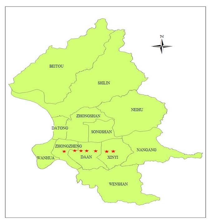
According to the website of the Department of Rapid Transit Systems, Taipei City Government,
the Xinyi line runs from Chiang Kai-shek Memorial Hall MRT station along Xinyi Road to the Xinyi
Planning District, crossing Jinhua Street, Aiguo East Road, and Hangzhou South Road and ending in
Xiangshan Park. The line spans 6.4 km with seven underground stations, including Xiangshan Station,
Taipei 101/World Trade Center Station, Xinyi Anhe Station, Daan Station, Daan Park Station, and
Chiang Kai-shek Memorial Hall Station. The entire line was constructed underground (Figure 1).
3.2. Sample Statistics
Table 2 provides statistics for the transaction data sample related to the beginning of metro
construction.
REAL ESTATE MANAGEMENT AND VALUATION, eISSN: 2300-5289 33
vol. 28, no. 1, 2020www.degruyter.com/view/j/remav
Stars indicate stations
Fig. 1. Taipei Metro Xinyi Line route map. Source: own study.
Table 2
Sample statistics: Beginning of construction as the division time point (N=2,315)
Unit of
Variable Mean SD Max. Min.
Measurement
PRICE 1103.53 560.330 6800 135 NT$10,000
AGE 23.00 8.992 43 0 Years
TYPE 0.60 - 1 0 -
ROOM 2.79 0.894 5 1 Rooms
LIVROOM 1.85 0.384 3 1 Rooms
BATH 1.58 0.493 2 1 Rooms
FLOOR1 0.06 - 1 0 -
FLOOR4 0.21 - 1 0 -
34 REAL ESTATE MANAGEMENT AND VALUATION, eISSN: 2300-5289
vol. 28, no. 1, 2020www.degruyter.com/view/j/remav
Source: own study.
Table 3 provides statistics for the transaction data sample related to the beginning of metro
operation.
Table 3
Sample statistics: Beginning of operation as the division time point (N=2,266)
Unit of
Variable Mean SD Max. Min.
Measurement
PRICE 2378.37 1442.626 33,300 410 NT$10,000
AGE 23.78 10.293 48 0 Years
TYPE 0.72 - 1 0 -
ROOM 2.70 0.960 9 1 Rooms
LIVROOM 1.80 0.460 6 1 Rooms
BATH 1.62 0.574 7 1 Rooms
FLOOR1 0.06 - 1 0 -
FLOOR4 0.16 - 1 0 -
Source: own study.
4. Empirical Results
Spatial dependence was tested first. In this study, global spatial autocorrelation coefficients were used
in the spatial econometric model to measure spatial autocorrelation. The calculation of global spatial
autocorrelation requires that the spatial neighborhood within the research range be defined.
Autocorrelation coefficients are derived from the spatial weights matrix. In this study, queen
contiguity was set as the contiguity weight to examine whether spatial aggregation was present in
housing prices. Moran’s I reached the 1% significance level at the beginning of metro construction,
indicating the presence of autocorrelation between neighborhood housing prices. The presence of
aggregation needed to be tested using spatial models. LM-lag and LM-error values reached the 1%
significance level. The robust LM-lag value was 56.325, reaching the 5% significance level. The robust
LM-error value was 2.422, not reaching the significance level. With regard to metro operation,
Moran’s I was 0.2551, reaching the 1% significance level and indicating positive autocorrelation
between housing prices. The presence of aggregation needed to be tested using spatial models. LM-lag
and LM-error values reached the 1% significance level. The robust LM-lag value was 56.851, reaching
the 1% significance level. The robust LM-error value was 29.149, reaching the 1% significance level.
The results indicated the presence of autocorrelation between neighborhood housing prices and error
terms.
This study compared calculations based on OLS, the spatial lag model, and the spatial error model.
Regression analyses are provided in Table 4. The Breusch-Pagan test was performed to test the three models
for residual heterogeneity; the results related to the beginning of metro construction reached the 1%
significance level, indicating rejection of the heterogeneity null hypothesis in all three models and, thus,
2
indicating the presence of residual heterogeneity in the regression models. The R values of the three models
were 0.389, 0.434, and 0.431, respectively. The spatial lag model was found to explain most variance. Log
likelihood, AIC, and SC values were used to indicate the goodness of fit of model estimation results. Higher
log likelihood values were associated with lower AIC and SC coefficients and better goodness of fit. Log
likelihood values of the models were -1338.05, -1270.2, and -1280.709, respectively. AIC values of the models
REAL ESTATE MANAGEMENT AND VALUATION, eISSN: 2300-5289 35
vol. 28, no. 1, 2020www.degruyter.com/view/j/remav
were 2700.1, 2566.41, and 2585.42, respectively. SC values of the models were 2769.06, 2641.12, and 2654.38,
respectively. The results indicated that the spatial lag model had the best goodness of fit. Breusch-Pagan
results related to the beginning of metro construction reached the 1% significance level, indicating rejection of
the heterogeneity null hypothesis in all three models and, thus, indicating the presence of residual
2
heterogeneity in the regression models. The R values of the three models were 0.357, 0.475, and 0.480,
respectively. The spatial error model was found to explain most of the variance. With regard to the goodness
of fit results, log likelihood values of the models were -1495.16, -1311.98, and -1316.54, respectively. AIC
values of the models were 3014.32, 2649.96, and 2657.08, respectively. SC values of the models were 3083.03,
2724.39, and 2725.79, respectively. The results indicated that the spatial error model had the best goodness of
fit.
The spatial lag and error model results are described here. With regard to housing structural
characteristics when the beginning of metro construction was set as the division time point, the age of
building coefficient was -0.023, reaching the 1% significance level. The coefficient of the age of the building
squared was 0.001, reaching the 1% significance level. These results indicated that an older age of building
was associated with lower housing prices; the rate of such a decrease in prices was smaller for older
buildings. Coefficients of the number of rooms were 0.196 and 0.200, reaching the 1% significance level, which
indicated that the housing price increased by 19.6% and 20.0% with each additional room, respectively.
Coefficients of the number of living rooms were 0.212 and 0.217, reaching the 1% significance level, which
indicated that the housing price increased by 21.2% and 21.7% with each additional living room, respectively.
Coefficients of the number of bathrooms were 0.218 and 0.214, reaching the 1% significance level, which
indicated that the housing price increased by 21.8% and 21.4% with each additional bathroom, respectively.
The housing type coefficients were 0.217 and 0.194, reaching the 1% significance level, which indicated that
housing prices in multistoried buildings and mansions were 21.7% and 19.4% higher than those in apartment
buildings. The coefficients of the location on the first floor were 0.177 and 0.176, reaching the 1% significance
level, which indicated that prices of housing units located on the first floor were 17.7% and 17.6% higher than
those of housing units on other floors. Coefficients of the location on the fourth floor were -0.012 and -0.008,
indicating a negative effect but not reaching the significance level. With regard to housing structural
characteristics, when the commencement of metro operation was set as the division time point, the obtained
coefficients were similar to those related to the beginning of metro construction in terms of direction and
significance and, thus, are not discussed here.
With regard to DD variables, the coefficient of MRT construction commencement time was 0.229, reaching
the 1% significance level. The results indicated that regardless of the distance between housing units and
metro stations, housing prices increased by 22.9% after the beginning of metro construction. Coefficients of
the MRT influence range were 0.114 and 0.165, reaching the 1% significance level. The results indicated that
when the time of the beginning of metro construction was not considered, housing prices within the MRT
influence range were 11.4% and 16.5% higher than those outside this range.
Coefficients of the interaction variable of the construction commencement time and the metro influence
range were -0.079 and -0.091, reaching the 10% and 5% significance levels, respectively. These results
indicated that after the commencement of metro construction, housing prices within the metro influence
range (experimental group) decreased by 7.9% and 9.1% as compared to those outside the metro influence
range (control group).
The coefficients of the metro operation beginning time were 0.104 and 0.129, reaching the 1% significance
level, which indicated that, regardless of the distance between housing units and metro stations, housing
prices after the beginning of metro operation were 10.4% and 12.9% higher than those before the beginning of
metro operation. The coefficients of the metro influence range were 0.087 and 0.137, reaching the 1%
significance level, which indicated that, when the time of the beginning of metro operation was not
considered, housing prices within the metro influence range were 8.7% and 13.7% higher than those outside
this range. The coefficients of the interaction variable of operation beginning time and the metro influence
range were 0.003 and 0.010, indicating a positive effect but not reaching the significance level. The results
indicated that there was no significant difference between housing prices within and outside the metro
influence range after the beginning of metro operation.
With regard to spatial econometric models, spatial lag coefficients in the 500-meter spatial lag
model were 0.373 and 0.474, reaching the 1% significance level, which indicated that housing prices
were affected by neighborhood housing prices. Spatial error coefficients in the spatial error model
36 REAL ESTATE MANAGEMENT AND VALUATION, eISSN: 2300-5289
vol. 28, no. 1, 2020www.degruyter.com/view/j/remav
were 0.434 and 0.539, reaching the 1% significance level, which indicated spatial autocorrelation
between error terms due to confounding factors.
Table 4
Analysis of empirical results
Construction Operation
Variables
OLS SLM SEM OLS SLM SEM
Independent Coefficient Coefficien Coefficien Coefficient Coefficien Coefficient
variable (t value) t (t value) t (t value) (t value) t (t value) (t value)
5.479*** 3.019*** 5.599*** 6.414*** 2.986*** 6.592***
Intercept
(91.267) (13.457) (89.921) (125.893) (16.864) (123.763)
-0.023*** -0.023*** -0.023*** -0.010*** -0.013*** -0.010***
AGE (-6.232) (-6.439) (-6.000) (-2.648) (-3.955) (-2.738)
0.001*** 0.001*** 0.001*** 0.001 0.001** 0.001
AGE 2 (5.486) (5.154) (4.482) (1.525) (2.058) (0.930)
0.199*** 0.196*** 0.200*** 0.210*** 0.201*** 0.203***
ROOM
(14.805) (15.134) (15.280) (14.056) (14.921) (15.169)
0.213*** 0.212*** 0.217*** 0.138*** 0.131*** 0.141***
LIVROOM
(7.629) (7.861) (8.041) (5.034) (5.262) (5.747)
0.235*** 0.218*** 0.214*** 0.225*** 0.196*** 0.193***
BATH (10.020) (9.633) (9.367) (9.631) (9.293) (9.117)
0.273*** 0.217*** 0.194*** 0.222*** 0.148*** 0.109***
TYPE (12.315) (10.072) (8.309) (9.809) (7.211) (4.977)
0.164*** 0.177*** 0.176*** 0.068* 0.097*** 0.129***
FLOOR1 (4.283) (4.820) (4.820) (1.662) (2.639) (3.556)
-0.017 -0.012 -0.008 -0.064** -0.054** -0.052**
FLOOR4
(-0.731) (-0.548) (-0.360) (-2.346) (-2.171) (-2.144)
0.237*** 0.229*** 0.229*** 0.094*** 0.104*** 0.129***
TIMEt
(11.127) (11.143) (11.090) (3.528) (4.324) (5.415)
0.174*** 0.114*** 0.165*** 0.170*** 0.087*** 0.137***
MRTi
(5.109) (3.439) (3.942) (6.141) (3.450) (3.327)
TIMEt MRTi -0.077* -0.079* -0.091** 0.005 0.003 0.010
(-1.709) (-1.815) (-2.073) (0.080) (0.048) (0.180)
Spatial Lag -
0.373***
(11.451)
- -
0.474***
(20.014)
-
0.434*** 0.539***
Lambda( ) - - - -
(11.515) (20.477)
Breusch-Pagan 50.167*** 49.595*** 49.833*** 82.310*** 37.050*** 48.428***
Log likelihood -1338.05*** -1270.2*** -1280.709*** -1495.16*** -1311.98*** -1316.538***
SC 2769.06 2641.12 2654.38 3083.03 2724.39 2725.79
AIC 2700.1 2566.41 2585.42 3014.32 2649.96 2657.08
R2 0.389 0.434 0.431 0.357 0.475 0.480
Note: ***, **, and * indicate that the coefficient reaches the 1%, 5%, and 10% significance level, respectively, and is
significantly different from 0. Coefficient values are not standardized.
Source: own study.
5. Conclusion and Suggestions
This study explored one type of YIMBY facilities, namely, metro stations. The metro had different
influences on housing prices at the beginning of construction, completion of construction, and
beginning of operation (GE et al., 2012). The metro influence time points in this study included the
commencement of construction and commencement of operation. The empirical results demonstrated
that MRT had a different influence on neighborhood housing prices in these two phases.
REAL ESTATE MANAGEMENT AND VALUATION, eISSN: 2300-5289 37
vol. 28, no. 1, 2020www.degruyter.com/view/j/remav
This study considered the issue of potential spatial dependence between housing prices, which may
be ignored in the OLS model. As failure to solve the issue of spatial dependence can cause bias in
model estimation coefficients (CHEN HAYNES, 2015), this study used spatial econometric models to
solve the issue. Prior to the empirical analyses, Moran’s I was used to test spatial correlation within
the research range in order to verify whether there was spatial autocorrelation between housing prices
in Taipei. Moran’s I was equal to 0.214 for the commencement of metro construction and 0.290 for the
commencement of metro operation, reaching the 1% significance level. The results indicated the
presence of positive spatial autocorrelation between housing prices in Taipei, as well as their
aggregation.
The empirical results of the spatial lag model showed that the DD coefficient of the 500-meter
influence range in the beginning of metro construction was -0.079, reaching the 10% significance level.
The results indicated that housing prices within the 500-meter influence range decreased by 7.9% after
the beginning of metro construction. Traffic inconveniences, due to metro construction and
environmental externalities caused by dust from construction work had a negative effect on
neighborhood housing prices. With regard to related studies, GE et al. (2012) found that the beginning
of metro station construction had a significant negative effect on housing prices. SU (2011) and YANG
(2007) suggested that environmental externalities, noise issue, congestion issue, and the “dark age” of
traffic caused by metro construction can negatively affect housing prices. GENG et al. (2015) found that
THSR stations negatively affected housing prices within the specified range, potential reasons for
which were traffic jams, electromagnetic radiation pollution, noise, and crime rates near THSR
stations.
With regard to metro operation, DD coefficients of the 500-meter influence range were 0.003 and
0.058, indicating positive but insignificant effects. The results showed that metropolitan transport did
not significantly affect housing prices within the 500-meter influence range after the beginning of its
operation. These results could be related to the ”dark age” of traffic and noise caused by metro
construction. Furthermore, this could follow the overreaction to the announcement of metro station
construction. Due to the need for testing and governmental approval of the line, the Xinyi line was
introduced into service only three years after completion of its construction. This study suggested that
psychological anticipation could lead to the growth of neighborhood housing prices after completion
of metro construction and prior to the official beginning of metro operation. MCDONALD and OSUJI
(1995) found that land prices increased prior to metro operation due to psychological anticipation.
According to the empirical findings reported by BAE et al. (2003), metropolitan transport already had a
significant effect on housing prices even before the beginning of its service. FERGUSON, GOLDBERG and
MARK (1988) indicated that urban transit influenced the real estate market and housing prices before
system operations began, which was due to psychological anticipation.
The announcement, construction, and introduction of a metro line into service usually take several
years. This study was limited to exploring the influence of metro stations on neighborhood housing
prices after the commencement of metro construction and after the commencement of metro
operation. The effects of the metro stations on neighborhood housing prices in the planning,
announcement, and construction completion phases were not discussed. Moreover, data used in this
study only included housing transactions. Therefore, the influence of the Xinyi line on prices of other
real estate types, for example, commercial real estate, was not explored. With regard to the influence
range definition, it is suggested that future studies apply different distances when determining the
experimental group in order to analyze the influence of metro stations on housing prices in different
zones.
References
Agostini, C. A., & Palmucci, G. A. (2008). The anticipated capitalisation effect of a new metro line on
housing prices. Fiscal Studies, 29(2), 233–256. https://doi.org/10.1111/j.1475-5890.2008.00074.x
Armstrong, R., & Rodriguez, D. (2006). An evaluation of the accessibility benefits of commuter rail in
eastern Massachusetts using spatial hedonic price functions. Transportation, 33(1), 21–43.
https://doi.org/10.1007/s11116-005-0949-x
Bae, C. H., Jun, M. J., & Park, H. (2003). The impact of Seoul’s subway line 5 on residential property
values. Transport Policy, 10(2), 85–94. https://doi.org/10.1016/S0967-070X(02)00048-3
Billings, S. B. (2011). Estimating the value of a new transit option. Regional Science and Urban Economics,
41(6), 525–536. https://doi.org/10.1016/j.regsciurbeco.2011.03.013
38 REAL ESTATE MANAGEMENT AND VALUATION, eISSN: 2300-5289
vol. 28, no. 1, 2020www.degruyter.com/view/j/remav
Bowes, D. R., & Ihlanfeldt, K. R. (2001). Identifying the impacts of rail transit stations on residential
property values. Journal of Urban Economics, 50(1), 1–25. https://doi.org/10.1006/juec.2001.2214
Boymal, J., de Silva, A., & Liu, S. (2013) Measuring the preference for dwelling characteristics of
Melbourne: Railway stations and house prices. 19th Annual Pacific Rim Real Estate Society Conference:
Future Directions : A Time of Change, 13-16.
Cervero, R., & Duncan, M. (2002). Benefits of proximity to rail on housing markets: Experiences in
Santa Clara County. Journal of Public Transportation, 5(1), 1–18. https://doi.org/10.5038/2375-
0901.5.1.1
Chen, Z., & Haynes, K. E. (2015). Impact of high speed rail on housing values: An observation from
the Beijing- Shanghai line. Journal of Transport Geography, 43, 91–100.
https://doi.org/10.1016/j.jtrangeo.2015.01.012
Dewees, D. N. (1976). The effect of a subway on residential property values in Toronto. Journal of
Urban Economics, 3(4), 357–369. https://doi.org/10.1016/0094-1190(76)90035-8
Diao, M., Leonard, D., & Sing, T. F. (2017). Spatial-difference-in-differences models for impact of new
mass rapid transit line on private housing values. Regional Science and Urban Economics, 67, 64–77.
https://doi.org/10.1016/j.regsciurbeco.2017.08.006
Dubé, J., Thériault, M., & Rosiers, F. (2013). Commuter rail accessibility and house values: The case of the
Montreal south shore, Canada, 1992-2009. Transportation Research Part A, Policy and Practice, 54, 49–66.
https://doi.org/10.1016/j.tra.2013.07.015
Dubin, R. A. (1998). Predicting house prices using multiple listings data. The Journal of Real Estate
Finance and Economics, 17(1), 35–59. https://doi.org/10.1023/A:1007751112669
Dziauddin, M. F., Alvanides, S., & Powe, N. (2013). Estimating the effects of light rail transit (LRT) system
on property values in Klang valley, Malaysia: A hedonic house price approach. Journal Technology,
61(1), 35–47. https://doi.org/10.11113/jt.v61.1620
Feng, C. M., Tseng, P. Y., & Wang, G. F. (1994). Impact of rail rapid transit system on housing price in
the station area. Journal of City and Planning, 21(1), 25–45.
Ferguson, B., Goldberg, M., & Mark, J. (1988). The pre-service impacts of the Vancouver advanced
light rail transit system on single family property values. In J. M. Clapp & S. D. Messner (Eds.), Real
Estate Market Analysis: Methods and Applications, 78–110. Greenwood Publishing Group.
Ge, X. J., Macdonald, H., & Ghosh, S. 2012, Assessing the impact of rail investment on housing prices
in North-West Sydney, 18th Annual Pacific-Rim Real Estate Society Conference, 15-18.
Geng, B., Bao, H., & Liang, Y. (2015). A study of the effect of a high-speed rail station on spatial
variations in housing price based on the hedonic model. Habitat International, 49, 333–339.
https://doi.org/10.1016/j.habitatint.2015.06.005
Gibbons, S., & Machin, S. (2005). Valuing rail access using transport innovations. Journal of Urban
Economics, 57(1), 148–169. https://doi.org/10.1016/j.jue.2004.10.002
Kopczewska, K., & Lewandowska, A. (2018). The price for subway access: Spatial econometric
modelling of office rental rates in London. Urban Geography, 39(10), 1528–1554.
https://doi.org/10.1080/02723638.2018.1481601
McDonald, J. F., & Osuji, C. I. (1995). The effect of anticipated transportation improvement on
residential land values. Regional Science and Urban Economics, 25(3), 261–278.
https://doi.org/10.1016/0166-0462(94)02085-U
McMillen, D. P., & McDonald, J. (2004). Reaction of house prices to a New Rapid Transit Line:
Chicago’s Midway Line, 1983–1999. Real Estate Economics, 32(3), 463–486.
https://doi.org/10.1111/j.1080-8620.2004.00099.x
Ryan, S. (2005). The value of access to highways and light rail transit: Evidence for industrial and
office firms. Urban Studies (Edinburgh, Scotland), 42(4), 751–764.
https://doi.org/10.1080/00420980500060350
Su Y.L. (2011). Assessing the value impacts of Taichung MRT stations on residential house market, National
Chi Nan University, Nantou County.
Tobler, W. R. (1970). A computer movie simulating urban growth in the Detroit region. Economic
Geography, 46, 234–240. https://doi.org/10.2307/143141
Trojanek, R., & Gluszak, M. (2018). Spatial and time effect of subway on property prices. Journal of
Housing and the Built Environment, 33(2), 359–384. https://doi.org/10.1007/s10901-017-9569-y
REAL ESTATE MANAGEMENT AND VALUATION, eISSN: 2300-5289 39
vol. 28, no. 1, 2020www.degruyter.com/view/j/remav
Wen, H., Gui, Z., Tian, C., Xiao, Y., & Fang, L. (2018). Subway opening, traffic accessibility, and
housing prices: A quantile hedonic analysis in Hangzhou, China. Sustainability, 10, 2254.
https://doi.org/10.3390/su10072254
Yang S.T., 2007, The housing price is influenced by the mass transit Neihu line, National Central University,
Taoyuan City.
Yiu, C. Y., & Wong, S. K. (2005). The effects of expected transport improvements on housing prices.
Urban Studies (Edinburgh, Scotland), 42(1), 113–125.
https://doi.org/10.1080/0042098042000309720
40 REAL ESTATE MANAGEMENT AND VALUATION, eISSN: 2300-5289
vol. 28, no. 1, 2020You can also read


