Design of control system for a 70 kA high temperature superconductor current lead - Prof. Dr.-Ing. Wolfgang Stief
←
→
Page content transcription
If your browser does not render page correctly, please read the page content below

Design of control system for
 a 70 kA high temperature
superconductor current lead

        Prof. Dr.-Ing. Wolfgang Stief

  University of Applied Sciences, Frankfurt/M
       Discipline of Control engineering

          Ausgabe: December 2, 2005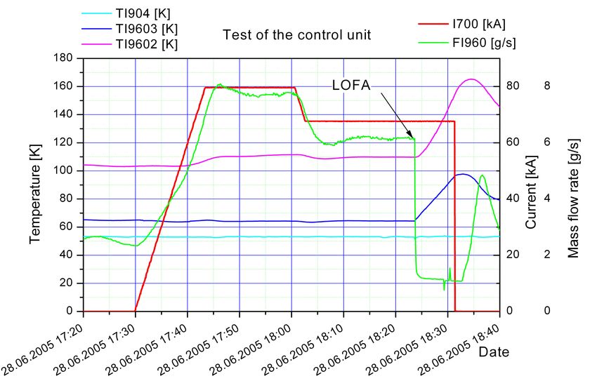
Contents
1 Introduction                                                                              1

2 Plant to control                                                                          1
  2.1 Design of the HTS current lead . . . . . . . . . . . . . . . . . . . . . . . . .      1
  2.2 Cryogenic cooling system . . . . . . . . . . . . . . . . . . . . . . . . . . . . .    2

3 Control system of the HTS current lead                                                    4

4 Identification                                                                            5

5 Modelbuilding of the HTS-Modul                                                            8

6 Structur of feedback system                                                              10

7 Structur of controller                                                                   12

8 Control facilities                                                                       13
  8.1 Hardware . . . . . . . . . . . . . . . . . . . . . . . . . . . . . . . . . . . . .   13
  8.2 Implemented Software . . . . . . . . . . . . . . . . . . . . . . . . . . . . . .     14

9 Measured cooling dynamic                                                                 17

10 Outlook: Inclusion of Thd                                                               18

11 Conclusion                                                                              19

12 Acknowledgement                                                                         21

                                              1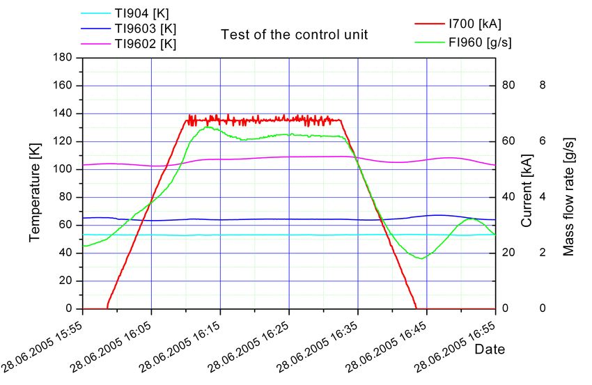
Abstract

This article describes the application of classical control theory to a cooling problem, the
temperature and mass flow control for a 70 kA high temperature superconductor current
lead. After identification and modelling a control system was developed, implemented and
tested. Furthermore, an empirical extension of the control structure is discussed, which may
take effect in special operational states of the current lead, e.g. to protect the head of the
current lead from to low temperature.
1     Introduction
In the frame of the European Fusion Technology Programme, the Forschungszentrum Karl-
sruhe has developed and built a 70 kA demonstrator current lead for the ITER Toroidal
Field (TF) coils using High Temperature Superconductors (HTS). The coolant mass flow
rate through the heat exchanger of the current lead has to be controlled in order to keep
the low temperature part with the HTS module superconducting, the high temperature part
above freezing temperature (because of the connected water cooled cables) and the mass
flow rate as low as possible. Up to now the mass flow rate of up to 4 installed current leads
is controlled manually by an experienced operator. For future experiments like ITER with
18 current leads only for the TF coils the mass flow rate and the temperature profile have
to be controlled automatically and an appropriate control system was developed, tested and
optimised.

2     Plant to control
2.1    Design of the HTS current lead
The three main parts of HTS-CL are the cold end clamp contact, the HTS module and the
heat exchanger as shown in a schematic cross section in Fig. 1 including the most important
temperature and mass flow sensors for the control system. The cold end clamp contact is

Figure 1: CAD view of the HTS current lead and schematic view of the 70 kA HTS module

cooled by the connected bus bar system, the HTS module is conduction cooled also from the
bus bar and the HEX is designed for He cooling with a temperature of 50 K. The HTS module
consists of the HTS part and two copper end caps, to provide the current transfer to the other
parts of the current lead. The connection to the copper terminal, which performs the clamp
contact to the bus bar, is done by soft soldering. The connection to the heat exchanger is

                                              1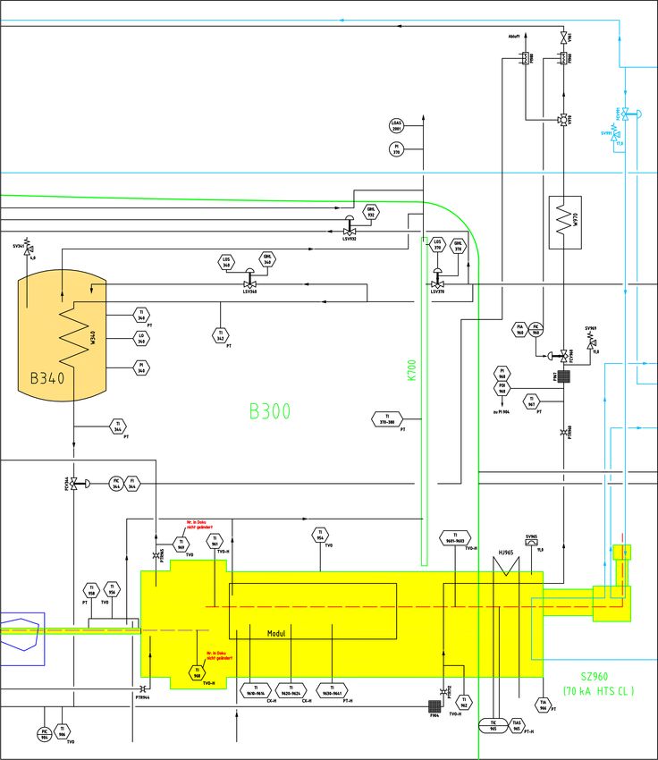
performed by a soft soldered screw contact for achieving low electrical resistance. The HTS
part is formed by 12 so-called panels. Each of them contain seven sintered stacks, made
of Bi-2223/AgAu tapes, soft soldered into stainless steel carriers with copper tips. More
details about the design and manufacturing of the lead are given in [1]. The installation

Figure 2: Overview of the integration of the HTS current lead into the vacuum vessel of
TOSKA

and integration into the vacuum vessel B300 of the TOSKA facility is shown in Fig. 2 as
overview and in Fig. 3 in detail.

2.2    Cryogenic cooling system
A 2 kW refrigerator was used for cool down, steady state operation and warm up of the test
arrangement. For the cool down, He was supplied directly from the refrigerator via transfer
line I (Fig. 4) to the test configuration in the vacuum vessel B300. During operation at 4.5
K the refrigerator liquefied into the control dewar (B250), and the bus bars were cooled in
a secondary cooling loop with supercritical He. The He needed for the conventional current
lead cooling was also supplied from this secondary cooling loop as shown in the simplified
flow scheme in Fig. 4. One piston pump and one centrifugal pump, installed in the control
cryostat (B250), circulated the He within this secondary loop. The refrigerator pressurized
the secondary cooling loop and replaced also the He subtracted for the current lead cooling.
In the case of the 4.5 K cooling of the HTS-CL, the He was also taken from the secondary
cooling loop.
For the HTS-CL operation in the temperature range between 50 K and 80 K, the He was
supplied directly from the 2 kW refrigerator via transfer line I. During this operation mode,
the He temperature could be stably adjusted at the desired value by the refrigerator.

                                             2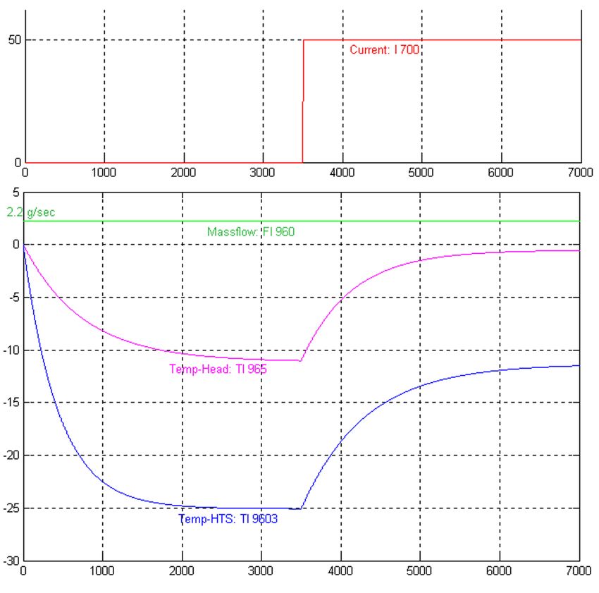
Figure 3: Detailed view of the HTS current lead into the vacuum vessel of TOSKA

For cooling the HTS-CL with LN2 , the sub-cooler B340 was required in order to feed the
HTS-CL with LN2 at a temperature of 77 K because the LN2 is supplied from a large storage
vessel with a supply pressure of 2.6 bar and an equivalent boiling temperature of 86.3 K.
The new developed control system of the HTS CL was tested with a He inlet temperature of
50 K which is the design temperature of the CL. In Fig. 5 a sub section of the detailed flow
diagram including all sensors required for operation and test of the HTS CL are shown.

       Figure 4: Simplified flow diagram of the cryogenic cooling system of TOSKA

                                             3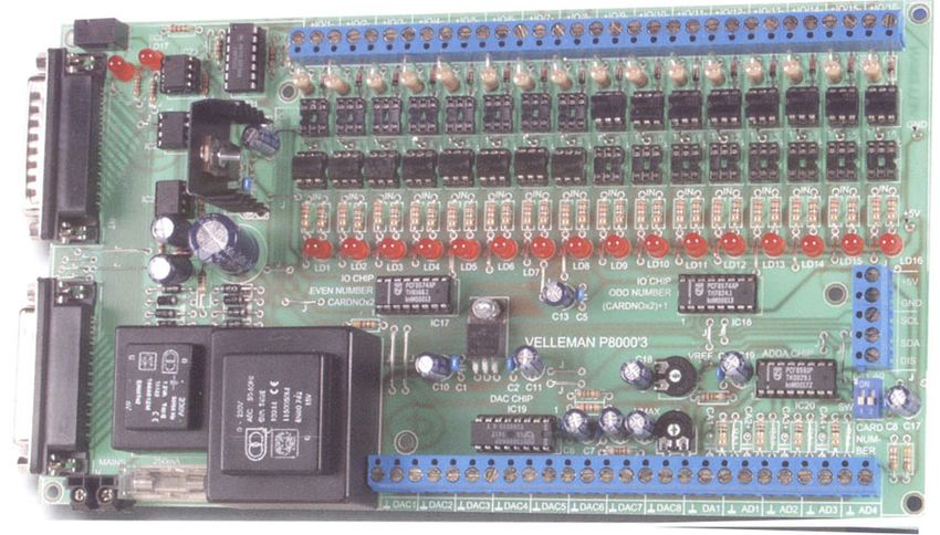
Figure 5: Sub section of the HTS CL part of the TOSKA flow diagram

3    Control system of the HTS current lead
The current lead is equipped with several temperature sensors as indicated in Fig. 4 and 5.
To control the temperature of the head, of the HEX and the HTS modul two of them (TI9603
at the HTS module side and TI965 at the warm end of the HEX) are used as control values
of the HTS CL. The temperatures are essentially influenced by the current I (I700) and the

                                            4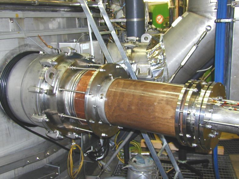
Figure 6: Abstract representation of the current lead as MIMO-System1
helium mass flow rate ṁhe (FI960) for cooling the current lead. So, the cooling system of
the HTS CL can be abstracted to a ”black box” with two inputs I and ṁhe and two outputs
Thd , Thts the temperatures at the head and the HTS-modul of the current lead, TI965 and
TI9603.
4 Identification
The design of a control system depends essentially of the dynamical behavior of the plant
to be controlled, which should be given in mathematical form. There are in principle two
ways to get it:
• theoretical modelbuilding
• experimental modelbuilding
In case of experimental analysis, i.e. ”identification”, the input- an output signals are mea-
sured to obtain a dynamical model, which will consist in case of the 2x2 current lead system
of four SISO-models (single input - single output), because each input will stimulate both
outputs. The development of an abstract model usually requires various simplifying assump-
tions of the plant. They will be:
• system can be considered to have ”lumped” parameters
• stochastical signals (e.g.noise) would be negligible
• the system responses would not depend on time, i.e. ”time-invariant system”
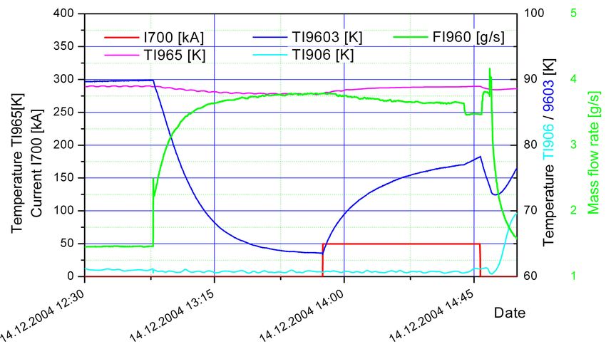
The experimental data are given as Fig. 7. The diagram shows that first ṁhe (mass flow,
green: FI960) increases (current remains zero) which decreases TI965 and TI9603 respec-
tively the temperatures of the head and HTS-Modul, Thd , Thts . When they are nearly steady
state the current I changes from 0 → 50kA (red line: I700) which increases the tempera-
tures.
The field of identification methods is widely spread. The characteristics of dynamical systems
can be obtained fundamentally by
• nonparametric methods
• parameter estimation methods
1
MIMO: multiple inputs-multiple outputs
5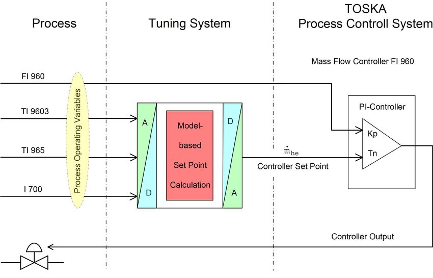
Figure 7: Measurement for system identification

where there are investigated about three times more parameter than nonparametric meth-
ods - in sum nearly twenty. The precision of parametric methods is much higher than the
other one, which can be realized even in graphical, manual way. For identification of the
current lead an algorithm of Golubev/Horowitz [2] is used which is implemented e.g. in
WINFACT98. Figure 8 shows the input-output relation between the mass flow ṁhe (brown
line) and the temperature at the head Thd extracted from Fig. 7, FI960 and TI965. These
datas must refered to zero initial values (Fig. 9) - if not, their initial values will be wrongly

                           Figure 8: Extracted input-output data

                                               6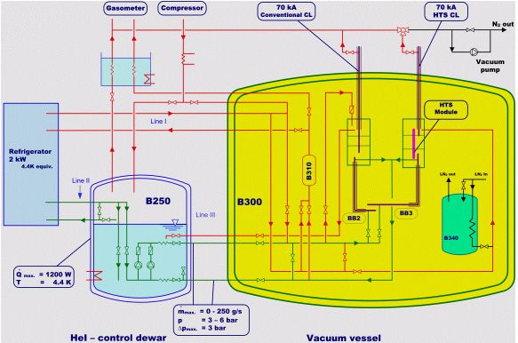
Figure 9: Input-output signals cleaned from initial condition

assumed as initial step. The input-output data are now readily treated for parameter esti-
mation by the mentioned algorithm. The output of the simulated model in Fig. 10 is shown
as full line, which can now easily calculated, because the parameter estimation procedure

                          Figure 10: Approximated output signal

is based onto the transfer function (Fig. 11). Yielding according to conventions of transfer
functions to
                                      Thd        −0.006697
                              G(s) =       =
                                      ṁhe    0.0013247 + 1 · s

                                             7
Figure 11: System identifying transfer function
or rather
Thd −5.055
G(s) =
=
ṁhe 1 + 754.9 s
to obtain the time constant T = 754, 9 sec. The remaining dynamical models are achieved
in similar way.
Thd −5.055
G11 (s) = = (1)
ṁhe 1 + 754.9 s
Thts −11.397
G12 (s) = = (2)
ṁhe 1 + 441.07 s
Thd 0.212
G21 (s) = = (3)
I 1 + 636.13 s
Thts 0.275 2
G22 (s) = = (4)
I 1 + 803.8 s
Represented as block diagramm (Fig. 12)
5 Modelbuilding of the HTS-Modul
Modellbuilding is an iterative process in generall: assumptions made in a first step have to be
verified in reality, modifications are necessary and yield to the next step . . . etc. Engineers,
physicists and other experts who are envolved with the present plant combine to get the best
2
Graphical identification method of all transfer functions yields to parameters of this order too. So
0.29
e.g. G22 (s) = 1+861.0 s
8Figure 12: Dynamical relations between the input-output signals of the current lead
model.
In this case a parallel structure is preferred, because it is assumed that the impact of the
mass flow would be much greater in changing the temperatures of the HTS modul and the
head although HTS and head are naturally mechanical coupled, which leads to thermical
interdependence. Same reflections concern the impact of the current and so the model of
the current lead will be:
Figure 13: Model of the current lead
The (linear) additive influence of the current is assumed because there will be only small
changes of states if feedback control is switched on. It has yet to be verified whether this linear
superposition is allowable when the plant will start up, i.e. current drives from 0 A → 80 kA.
An important feature of the plant can be viewed by the model concerning the structure
of control: it is only possible to control one of the two temperatures by the helium mass
flow! - either Thd or Thts . There is no second pipeline - no second ”actuator” - to control
independently head or HTS: the process to be controlled is said to be not ”completely
9controllable”.
The simulation diagram (Fig. 14) of the model matches well with the reality of Fig. 7 either
Figure 14: Simulation of the current lead
in the time constants or in the gain factor for steady state. An important step has done
for developing a controller, because a physical-mathematical model is the best condition to
develop
• the structur of the feedback system
• the structur of the controller and
• its parameters
6 Structur of feedback system
There is a well known difference between explorations of structures for feedback systems
and structures of controllers: there exist no theory respectively there are well established
methods and that´s because empirical knowledge is demanded to find an efficient feedback
structure.
The more important output to be controlled is the temperature of the HTS modul Thts ,
because it must be below a certain limit otherwise there is no superconductivity. Thd is
10dynamical coupled and will only be observed to prevent critical head temperatures i.e. the
algorithm of the choosen controller will be varied by Thd in some way.
The current I will be – in contrast to Fig. 6 – imposed from ”external” and will be interpreted
by this way as disturbance signal. Since I is measured it can be used for ”feedforward control”
using already existing relation (Fig. 15) between I and ṁhe for the operating point of the
current lead, i.e. 65 K ≤ Thts ≤ 70 K
Figure 15: Steady state mass flow for given current
With theses reflections the control concept yield to
Figure 16: Control structure for Thts with feedforward control
11An extension of this control concept for observing Thd will be discussed in chap. 10.
7 Structur of controller
The design of the controller for Thts will be based on the ”root locus method”, because -
in contrast to the ”frequency domain” - this method get deep insight into the dynamical
behaviour of the feedback system. It´s based on the open loop
−11.397
Fo (s) = FR (s) (5)
1 + 441.07 s
where FR (s) is the transfer function of the controller to be designed by special software e.g.
MATLAB-Simulink , M AT RIXx , DORAPC. By using the Simulink-SISO tool the design is
essentially done in operator interfaces as shown in Fig. 17. The structure of the controller is
Figure 17: Root locus design window
defined by the pole-zero configuration in red, which lead to the illustrated closed loop step
response and yield to the transfer function
˙
m(s) 1 + 330 s 0.003 + s
FR (s) = = KR = KR∗ (6)
e(s) s s
For determining the digital implementation of this analogue controller Tustin´s rule without
2(z − 1)
s→ (7)
TA (z + 1)
12prewarping - because the critical frequency is much lower than the Nyquist frequency - is
used. FR (s) yield to (TA = sample time = 2 sec.)
2(z−1)
0.003 + TA (z+1)
FR (z) = KR∗ 2(z−1)
TA (z+1)
1.003 − 0.997 z −1
FR (z) = KR∗
1 − z −1
and finally to the implemented difference equation
mk = mk−1 + KR∗ {−(1.003ek − 0.997ek−1 )}3 (8)
where mk is the control signal or plant input helium mass flow and ek = Tsp − Thts the
control error (”sp”: setpoint).
8 Control facilities
8.1 Hardware
The physical connection between the sensors for the inputs Thts , Thd , I the output mk and
the PC is realized by using a 8 bit, 0-5 V computer interface board (Fig. 18) which has a
Figure 18: K8000 interface board
simple connectionwith the printer port and communicate by the I 2 Cbus-protocol. The range
3
The negative sign before ”(” is due to the negative gain of the plant in equation 5.
13and solution of the input-output signals are
223 K ≤ Thd ≤ 323 K → 0.39 K/bit
50 K ≤ Thts ≤ 80 K → 0.12 K/bit
0 A ≤ I ≤ 80 kA → 0.31 kA/bit
g/sec
0 g/sec ≤ ṁhe ≤ 15.9 g/sec → 0.062
bit
There are no (low pass) filters needed on analogue inputs, because the sample frequency is
2π
2 sec
= πsec−1 and therefore the aliasing frequencies will be entirely attenuated by the plant´s
1
critical frequency [3] of about 441.07 = 0.0022 sec−1 what is also confirmed by simulation.
The hardware of the tuning system is embedded in the TOSKA facility as
Figure 19: Block diagram control loop
which shows that the mass flow ṁhe calculated by the control system doesn´t activate the
helium valve directly, but is the input for an always existing mass flow controller. When the
current lead has been identified the dynamic of this controller was involved.
8.2 Implemented Software
Equation 8 is embedded in initialisations, AD/DA-instructions and the repeat . . . until
keypressed - control loop to provide the sample rate of TA = 2 sec. The algorithm is
implemented in syntax of PASCAL 6.0 .
14PROGRAM SZFG-Regelung;
USES I2C, Crt, Dos;
Var i,Imk: Integer;
Tsoll,Tkopf,Kopfmin,ekopf,Tmitte,Tm_max,Strom,mk,mk_1,ek,ek_1,ek_2: real;
H, M, Sek, S100, Sek_alt: Word;
ch: Char;
shour,smin,ssek,stime,smk,sges,sTkopf,sTmitte,sStrom,sdaten: string;
f:text;
{------------------------------------}
BEGIN
ClrScr;
assign(f,’regler.dat’);
rewrite(f);
GetTime(H, M, Sek, S100);
i:=0;
Sek_alt := Sek;
mk_1 := 3.1;
ek_1 := 0;
ek_2 := 0;
Strom := 0;
Kopfmin := 260;
Tm_max := 5; {z.B. wenn Tsoll=60K, Tmitte=65K}
Write(’Sollwert Mittentemp.[K] = ’);
Read(Tsoll);
Repeat
GetTime(H, M, Sek, S100);
GotoXY(1,3);
writeln(’Sek:Sek100 = ’,Sek:2,’:’,S100:3);
IF Sek Sek_alt
THEN
begin
writeln(’i = ’,i:2);
IF i=2
THEN
begin
ReadADchannel(1);
ReadADchannel(2);
ReadADchannel(3);
{ReadADchannel(4);}
str(H:2, shour);
str(M:2, smin);
str(Sek:2, ssek);
stime := concat(shour,’:’,smin,’:’,ssek);
{Kalibrierung}
Tkopf := AD[1]*0.392+223; {ad[1]*100/255+223,d.h.223...323K}
Tmitte := AD[2]*0.118+50; {ad[2]*30/255+50,d.h.50...80K}
Strom := AD[3]*0.3137; {ad[3]*80kA/255 in kA}
ekopf := Tkopf - Kopfmin;
{Writeln(’AD1 ’,AD[1]:3);
Writeln(’AD2 ’,AD[2]:3);
Writeln(’AD3 ’,AD[3]:3);}
writeln;
Writeln(’Kopftemp.: ’,Tkopf:3:1);
15Writeln(’Mittentemp.: ’,Tmitte:3:1);
Writeln(’Strom: ’,Strom:6:1);
{Writeln(’AD channel 4 : ’,AD[4]:3);}
{Regeldifferenz}
ek := Tsoll - Tmitte;
writeln(’ek =’,ek);
{PI-Regler-Algorithmus}
mk := mk_1 - 1.003*ek + 0.997*ek_1;
mk_1 := mk;
ek_1 := ek;
{IF mk < 0 THEN mk := 0; z.B. beim Anfahren,therm.Dyn.bleibt}
writeln;
writeln(’mk aus Algo =’, mk:5:3);
{Störgrößenaufschaltungen (feedforward) für Strom und gegen Kopfmin-Unterschreitg.:
je näher Tkopf an 260 K, desto weniger He}
mk := mk + 0.07*Strom;
{IF -ek 0
THEN IF mk = 0
THEN mk := 0.091*Strom
ELSE mk := mk + 0.07*Strom - 2/(eKopf+2/mk)
ELSE mk := 0.07*Strom;
END
ELSE mk := mk + 0.07*Strom;}
{Begrenzung}
IF mk 15.9 THEN mk:=15.9;
writeln;
writeln(’mk in [g/sek] = ’,mk:5:3);
str(mk:4:2,smk);
mk := mk*16.038; {mk*255/15.9}
writeln(’mk in [Bit] = ’,mk:4:2);
Imk := Round(mk);
writeln(’Imk in Bits = ’, Imk:4);
OutputDAchannel(1,Imk);
str(Tkopf:3:5,sTkopf);
str(Tmitte:3:5,sTmitte);
str(Strom:3:5,sStrom);
sdaten := concat(smk,’ ’,sTkopf,’ ’,sTmitte,’ ’,sStrom);
sges := concat(stime,’ ’,sdaten);
append(f);
writeln(f,sges);
close(f);
i:=0;
end
ELSE begin i:=i+1; Sek_alt := Sek; end;
end;
until keypressed;
END.
169 Measured cooling dynamic
The test of the developed mass flow control system of the HTS current lead was included in
the ”HTS-CL Test Procedure HTS IV with LN2 cooling” 4 , scheduled on june 27-28. Test
objectives have been
• Test the behavior of the control system for the helium mass flow rate in steady state
operation with changes of the current in certain limits (10 kA)
• Test the behavior during rump up and down for 0 ↔ 50 kA ↔ 80 kA
• Optimize the parameter of the control system
Diagram 20 shows the control for current change I (I700) 80 kA → 68kA in operation mode
beginning at 18.00 o´clock, the reaction of the controller, the mass flow FI960, and the
HTS-temperature with setpoint = 65 K to be controlled, TI9603.
When current increases from 0 kA to 80 kA at 17.30 Thts can be hold within 64 K . . . 65 K.
Figure 20: Mass flow control: I changes 0 → 80 kA with following step down
Nearly the same transition of Thts occurs when current runs from 0 → 68kA (Fig. 21). When
current has reached its final value Thts – such as can be seen in Fig. 20 – the control error is
about 1%.
4
Draft in ver. 1.0, 6/1/2005
17Figure 21: Mass flow control: I changes 0 → 68 kA → 0
At 16.32 o‘clock the current lead is rump down with (unexpectedly) oscillating Thts and mass
flow, FI960. The oscillations are rather weak damped and should have to be answered, what
can be done by looking on Fig. 17. This diagram teaches: if the gain of the plant decreases,
the (complex) poles of the closed loop control circuit approach to the imaginary axes and
therefore the tendency of oscillations increases.
Obviously there are different gain factors of the current lead when it is rump up and down.
Normaly the identification procedure (chap. 4) should be done again with current-step-down
(e.g. 50 kA → 0) – a great amount on time and cost is caused. Therefore it is proposed to
enlarge empirically the gain factor of the controller what will compensate the smaller gain
of the plant and will lead to a damped cool-down behavior.
On the other way: no danger will be due by oscillations because there is no electrical energy
in the current lead if I = 0 A.
10 Outlook: Inclusion of Thd
The discussed control structure does not consider the temperature of the head Thd . As men-
tioned above (chap. 5) Thd is coupled with Thts and therefore not ”completely controllable”.
For most of controlled operating modes Thd is in uncritical range – especially not to cold
i.e. not below 260 K, which is achieved by adequate construction and is shown by diagrams
18Fig. 20 and 21.
Nevertheless the consisting control structure has been extend (green coloured blocks) to ob-
serve Thd and to manipulate the helium mass flow, i.e. the control signal, if Thd approaches
Figure 22: Extented control concept
1
to its minimum temperature: the closer Thd is to 260 K the higher is the amount of Ku in
Fig. 22, which will decrease the helium mass flow. In this way the head of the current lead
is protected against coldness. On the other side - especially if Thd remains in the near of its
minimum - Thts increases (because of less helium flow) until a fixed maximum, which has to
be set to guarantee the superconducting operating state 5 . If Thts obtains its maximum, the
Thd -extension will be switched off, because it is more important to stay in superconducting
state than to have a lower Thd .
11 Conclusion
This project helps to increase the automation for the operation of the 80 kA current lead,
which has been designed by the Forschungszentrum Karlsruhe for the European Fusion Tech-
nology Programme.
5
e.g. ϑhts,max = ϑsp + 5 K
19The development of the control system is based on typical ”lecture”-steps
• decision of actuators and sensors
• identification
• modellbuilding
• design of controller
• simulation and
• test phase
which are true to be theoretically well known but in practice the bottleneck is to find a
dynamical modell.
The identification run in december 2004 performed really satisfied, because the plant had
been placed in such a well experienced steady state that the actuators could be turned on
one after another to influence the outputs in such a way too – a precondition for yielding
decoupled dynamical relations. The calculated four mathematical-phyical models have all
P T1 -structur with relativ great time constants in the order of 500-1000 seconds, i.e. steady
states get about 1500-3000 seconds – nearly one hour and therefore a hint on careful design
of the controller because of the tendency of oscillations.6
An additiv superpositioned parallel structured model-connection was rather plausible and
matched very good to the measured process variables – the bottleneck was done!
On the basis of this well proved model the open loop transfer function to control Thts was
used to design the controller by the root locus method which yielded to a controller of
PI-type and parameters within rather narrow bounds (TI = 333.3 sec). The current has
been modelled as ”disturbance”-signal and could compensated by ”feedforward control”.
The discretisation of the PI-controller had been done by using Tustin´s formula and was
implemented in PASCAL.
On june of 28 the test of this mass flow control system achieved to a control error of 1%
in steady state ϑhts,sp = 65 K and of 2%-(oscillating)-error when current is switched from
0 → 80 kA. The deviations could be certainly improved, if there were more time for the test
phase. As a final conclusion it can be said that the developed control structur is ready to
be used in ITER.
6
The dynamical models could had been also identified as P DT1 -types but without relevant deviations or
improvements.
2012 Acknowledgement
The author thanks Mr. Gernot Zahn who has initiated this project and to his excellent crew
in the process control center, whose expertise, experience, ideas and nice atmosphere made
their own positiv contributions.
This project was very interesting for the author because it was the first time that he could
work neither at a typical laboratory facility in the order of an ”table” neither at a production
line (such as a mill train) but at a laboratory facility in the order of nearly a production line
- with the great advantage to make measurements with stop and goes, i.e. to work without
being forced to production. Moreover the background of fusion energy has been and will be
very interesting and will be joined with best wishes of much success in the future.
References
[1] R. Heller, D. Aized, A. Akhmetov, W.H. Fietz, F. Hurd, J. Kellers, A. Kienzler, A.
Lingor, J. Maguire, A. Vostner, R. Wesche, Design and Fabrication of a 70 kA Current
Lead using Ag/Au stabilized Bi-2223 Tapes as a Demonstrator for the ITER TF-Coil
System, IEEE Trans., Appl. Supercond., Vol 14, No. 2, June 2004, p. 1774-1777
[2] Boris Golubev, Isaac Horowitz, Plant rational transfer approximation from input-output
data, Int. Journal of Control, p. 711-723, 1982
[3] J. Golten, A. Verwer, Control of System Design an Simulation, McGraw-Hill, p. 293-296,
1991
21You can also read