A Learning Algorithm for Place Recognition
←
→
Page content transcription
If your browser does not render page correctly, please read the page content below
A Learning Algorithm for Place Recognition
                                                       César Cadena and José Neira

   Abstract— We present a place recognition algorithm for                      common technique used to enforce consistency in matches
SLAM systems using stereo cameras that considers both                          [2,4]. Recently proposed by Paul and Newman [6], the FAB-
appearance and geometric information. Both near and far                        MAP 3D uses the same FAB-MAP framework including 3D
scene points provide information for the recognition pro-
cess. Hypotheses about loop closings are generated using a                     information provided by a laser scanner for the distances
fast appearance technique based on the bag-of-words (BoW)                      between features, but can only make such inferences about
method. Loop closing candidates are evaluated in the context                   visual features in the laser range.
of recent images in the sequence. In cases where similarity is                    The algorithm for place recognition presented here, first
not sufficiently clear, loop closing verification is carried out               proposed in [7] and improved in [8], uses two complementary
using a method based on Conditional Random Fields (CRFs).
We compare our system with the state of the art using visual                   techniques. Candidate loop closing locations are generated
indoor and outdoor data from the RAWSEEDS project, and                         using an improved bag-of-words method (BoW) [1], which
a multisession outdoor dataset obtained at the MIT campus.                     reduces images to sparse numerical vectors by quantising
Our system achieves higher recall (less false negatives) for full              their local features. This enables quick comparisons among
precision (no false positives), as compared with the state of                  a set of images to find those which are similar. Hierarchical
the art. It is also more robust to changes in appearance of
places because of changes in illumination (different shadow                    implementation improves efficiency [9]. Hypothesis verifi-
configurations in different days or time of day). We discuss the               cation is based on CRF-Matching. CRF-Matching is a pro-
promise of learning algorithms such as ours, where learning                    babilistic model able to jointly reason about the association
can be modified on-line to re-evaluate the knowledge that the                  of features. It was proposed initially for 2D laser scans [10]
system has about a changing environment.                                       and monocular images [11]. The CRF infers over the scene’s
                         I. I NTRODUCTION                                      image and 3D geometry. Insufficiently clear loop closure
                                                                               candidates from the first stage are verified by matching the
   In this paper, we consider the problem of recognising
                                                                               scenes with CRFs. This algorithm takes advantage of the
locations based on scene geometry and appearance. This
                                                                               sequential nature of the data in order to establish a suitable
problem is particularly relevant in the context of environment
                                                                               metric for comparison of candidates, resulting in a highly
modeling and navigation in mobile robotics. Algorithms
                                                                               reliable detector for revisited places.
based on visual appearance are becoming popular to detect
                                                                                  The basic idea of the algorithm is to exploit the efficiency
locations already visited, also known as loop closures, be-
                                                                               of BoW for detecting revisited places in real-time and the
cause cameras are inexpensive, lightweight and provide rich
                                                                               higher robustness of CRF-Matching to ensure that revisiting
scene detail.
   Many methods focus on place recognition, and mainly use                     matches are correct. In order to keep the real time execution,
the bag-of-words representation [1], supported by some pro-                    only insufficiently clear results of BoW are input to CRF-
babilistic framework [2]. Techniques derived from BoW have                     Matching.
been successfully applied to loop closing-related problems                        In the next section we provide a description on our place
[2,3], but could exhibit false positives in cases when the same                recognition system. In section III we present experimental
features are detected although in a different geometric con-                   results on real data that demonstrate the improvement in
figuration. An incorrect loop closure can result in a critical                 robustness and reliability of our approach. Finally, in section
failure for SLAM algorithms. On the issue of recognition                       IV we discuss the results and discuss the applicability of our
of revisited places we consider the state of the art is the                    system to operations over time.
FAB-MAP [3]. It has proved very high precision although                                  II. T HE P LACE R ECOGNITION S YSTEM
with reduced recall. In other words, the low proportion of
false positives is attained by sacrificing many true positives                   The place recognition system [7,8] is a loop closing
[4]. This system also presents problems in applications using                  candidate generation-verification scheme. In this section, we
front facing cameras [5].                                                      describe both components of the system.
   To avoid mismatches in these appearance-based ap-                           A. Loop Candidates Detection
proaches, some geometrical constraint is generally added
                                                                                 The first component is based on the bag-of-words method
in a verification step. The epipolar geometry is the most
                                                                               (BoW) of [1] which is implemented in a hierarchical way,
   César Cadena and José Neira are with the Instituto de Investigación en   thus improving efficiency [9]. In this implementation we use
Ingenierı́a de Aragón (I3A), Universidad de Zaragoza, Zaragoza 50018,         64-SURF-features, see Fig. 1(a). λt is the BoW score com-
Spain. {ccadena, jneira}@unizar.es.
   This research has been funded by the Dirección General de Investigación   puted between the current image and the previous one. The
of Spain under projects DPI2009-13710, DPI2009-07130.                          minimum confidence expected for a loop closure candidate is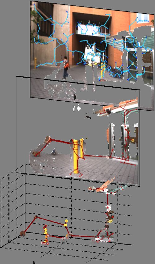
α− ; the confidence for a loop closure to be accepted without
further verification is α+ . The images from one session
are added to the database at one frame per second. This
implementation enables quick comparisons of one image at
time t with a database of images in order to find those that
are similar according to the score s. There are 3 possibilities:
   1) if s ≥ α+ λt the match is considered highly reliable
       and accepted;
   2) if α− λt < s < α+ λt the match is checked by CRF-
       Matching in the next step of verification.
   3) otherwise. the match is ignored.

B. Loop Closure Verification
   When further verification is required, loop closing candi-
                                                                                                  (a) BoW step
dates are verified for consistency in 3D and in image space
with CRF-Matching, an algorithm based on Conditional
Random Fields (CRF) [12]. CRF-Matching is a probabi-
listic graphical model for reasoning about joint association
between features of different scenes. We model the scene
with two graphs, the first one for SURF-features with 3D
information (near), and the second one over the remaining
SURF-features (far), see Fig. 1(b). The graph structure is
given for the minimum spanning tree over the euclidean
distances, either the 3D metric coordinates (G3D ) or 2D pixel
coordinates (GIm ). We use the CRF-Matching stage over the
loop closing candidates provided by the BoW stage. Then,
we compute the negative log-likelihood (Λ) from the MAP
associations between the scene in time t, against the loop
closing candidate in time t0 , Λt,t0 , and the scene in t − 1,
Λt,t−1 .
   The negative log-likelihood Λ3D of the MAP association
for G3D provides a measure of how similar two scenes are in
terms of close range, and ΛIm for GIm in terms of far range.
Thus, we compare how similar the current scene is with the
scene in t0 with respect to t − 1 with Λt,t0 ≤ βΛt,t−1 for
each graph. With the β parameters we can control the level
we demand of similarity to (t, t − 1), a low β means a high
demand. By choosing different parameters for near and far
information we can make a balance between the weight of
each in our acceptance. Our place recognition system can be
summarized in the algorithm 1.                                                                    (b) CRF step

                     III. E XPERIMENTS                             Fig. 1. Outdoor scene from the MIT campus. We get the SURF-features
                                                                   for the BoW stage over one image of the stereo pair 1(a). For the CRF stage
   We have evaluated our system with the public datasets           we compute the two minimum spanning trees (MST), one for features with
from the RAWSEEDS Project [13]. The data were collected            3D information (near features), and the second for the remaining ones, with
by a robotic platform in static and dynamic indoor, outdoor        image information (far features). In 1(b), we show the two resulting graphs:
                                                                   in blue the graph for far features (GIm ), in dark red the graph for near
and mixed environments. We have used the data correspond-          features (G3D ). We apply CRF-Matching over both graphs. The minimum
ing to the Stereo Vision System with an 18cm baseline.             spanning tree of G3D is computed according to the metric coordinates,
Images are (640x480 px) taken at 15 fps.                           projected over the middle image only for visualisation. In the bottom, we
                                                                   show G3D in metric coordinates with the 3D point cloud (textured) of each
   We used 200 images uniformly distributed in time, from          vertex in the tree. The MST gives us an idea of the dependencies between
a static mixed dataset taken on 01-Sep-2008, for training          features in a scene, and allows for robust consistency checks of feature
the vocabulary for BoW and for learning the weights for            associations between scenes.
CRF-Matching. In order to learn the weights for the CRF-
Matching, we obtained the SURF features from the right im-         time t−δt . The results from RANSAC were our labels. Since
age in the stereo system and computed their 3D coordinates.        the stereo system has high noise in the dense 3D information,
Then, we ran a RANSAC algorithm over the rigid-body                we selected δt = 1/15s. The same procedure is done over
transformation between the scene at time t and the scene at        the SURF features with no 3D information, where we obtain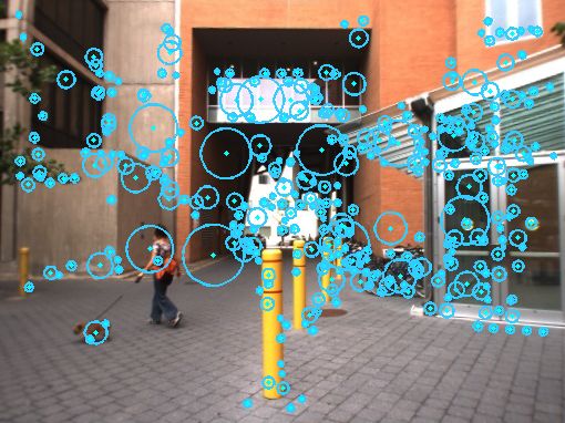
TABLE I
                                                  PARAMETERS FOR THE EXPERIMENTS

                                      FAB-MAP 2.0                                         Our System
                                         RAWSEEDS             MIT                        RAWSEEDS               MIT
                                  Indoor   Outdoor   Mixed   Campus                Indoor Outdoor Mixed        Campus
                 p                 50%      96%      62%      33%           α+      60%    60%       60%        60%
                 P (obs|exist)     0.31     0.39     0.37     0.39          α−      15%    15%       15%        15%
                 P (obs|!exist)    0.05     0.05     0.05     0.05          β3D       1     1.5       1.5        1.5
                 Motion Model       0.8      0.8      0.6      0.6          βIm      1.3    1.7       1.7        1.7

Algorithm 1 Pseudo-algorithm of our place recognition                 in order to obtain the best performance in each experiment.
system                                                                The parameters that we have modified are the following ones
Input: Scene at time t, Database h1, . . . , t − 1i                   (for further description please see [3] and [4]):
Output: Time t0 of the revisited place, or null
  Output = N ull                                                        •   p: Probability threshold. The minimum matching proba-
  Find the best score st,t0 from the query in the database of the           bility required to accept that two images were generated
  bag-of words                                                              from the same place.
  if st,t0 ≥ α+ st,t−1 then                                             •   P (obs|exist): True positive rate of the sensor. Prior
     Output = t0
                                                                            probability for detecting a feature given that it exists
  else
     if st,t0 ≥ α− st,t−1 then                                              in the location.
         Build the G3D and GIm                                          •   P (obs|!exist): False positive rate of the sensor. Prior
         Infer with CRFs and compute the neg-log-likelihoods Λ              probability for detecting a feature given that it does not
         if Λ3D            3D      Im            Im
              t,t0 ≤ β3D Λt,t−1 ∧ Λt,t0 ≤ βIm Λt,t−1 then                   exist in the location.
                         0
            Output = t                                                  •   Motion Model: Model Motion Prior. This biases the
         end if
     end if                                                                 matching probabilities according to the expected motion
  end if                                                                    of the robot. A value of 1.0 means that all the probability
  Add current scene to the Database                                         mass goes forward, and 0.5, means that probability goes
                                                                            equally forward and backward.
                                                                      In both systems, our and FAB-MAP, we disallow the matches
the labels by calculating with RANSAC the fundamental                 with frames in the previous 20 seconds. The final values
matrix between the images. Thus, we obtained a reliable               used by us are shown in Table I. We have chosen the
enough labelling for the training. Although this automatic            parameter set in order to obtain the maximum possible recall
labelling can return some outliers, the learning algorithm has        at one hundred percent precision. All the place recognition
demonstrated being robust in their presence. Afterwards, we           experiments are carried out at 1 fps.
tested the whole system in three other datasets: static indoor,
static outdoor and dynamic mixed. The four datasets were                                           TABLE II
collected on different dates and in two different campuses.                               R ESULTS FOR ALL DATASETS
Refer to the RAWSEEDS Project [13] for more details. In
                                                                                                          Precision   Recall
the fig. 2 we show the ground truth trajectories and results.                     RAWSEEDS
   For the first bag-of-words stage, we have to set the                           Outdoor (04-Oct-2008)
minimum confidence expected for a loop closure candidate,                                     FAB-MAP      100%       3.82%
                                                                                              BoW-CRF      100%       11.15%
α− , and the minimum confidence for a trusted loop closure,                       Mixed (06-Oct-2008)
α+ . We selected the working values α− = 15% and                                              FAB-MAP      100%       13.47%
α+ = 60% in all experiments. Since these datasets are                                         BoW-CRF      100%       35.63%
                                                                                  Indoor (25-Feb-2009)
fairly heterogeneous, we think these values can work well in                                  FAB-MAP      100%       26.12%
many situations. As It might depend on the datasets and the                                   BoW-CRF      100%       58.21%
vocabulary size, though. Then, for the CRF-Matching stage,                        Multisession MIT
we set the β parameters in order to obtain 100% precision.                        19-20 of July/2010
                                                                                              FAB-MAP      100%       38.89%
This allows comparisons with alternative systems in terms                                     BOW-CRF      100%       38.27%
of reliability. All the parameters used are shown in Table I.
   We have compared the results from our system against the
                                                                         The results of our system and of FAB-MAP over the
state-of-the-art technique FAB-MAP 2.0 [4]. The FAB-MAP
                                                                      RAWSEEDS datasets are shown in Fig. 2, and the statistics
software1 provides some predefined vocabularies. We have
                                                                      in Table II.
used the FAB-MAP indoor vocabulary for the RAWSEEDS
                                                                         In the outdoor dataset, FAB-MAP does not detect all the
indoor dataset and the FAB-MAP outdoor vocabulary for the
                                                                      loop closures zones, as shown in Fig. 2(a). The biggest loop
others datasets. This technique has a set of parameters to tune
                                                                      is missed in the starting and final point of the experiment,
  1 The software and vocabularies were downloaded from http://www.    in the top-right area of the map. One sample of this false
robots.ox.ac.uk/˜mobile/                                              negative area is shown in Fig. 3(a). The result of our system
Outdoor (04-Oct-2008)

                                               (a)                                                    (b)
                  Mixed (06-Oct-2008)

                                               (c)                                                    (d)
                  Indoor (25-Feb-2009)

                                               (e)                                                    (f)

Fig. 2. Loops detected by each of the methods in the RAWSEEDS datasets. On the left results from FAB-MAP and on the right results from our system
BoW + CRF-Matching. Black lines and triangles denote the trajectory of the robot; light green lines, actual loops, deep blue lines denote true loops
detected.
is shown in Fig. 2(b). At 100% of precision we can detect
all the loop closure areas.
For the experiment in the dynamic mixed environment we
get 100% precision with both systems. Though the recall is
lower in the FAB-MAP, see table II. Furthermore, all the
loop closure zones are not detected, see Fig. 2(c), with false
negatives as shown in Fig. 3(c), as compared with our results,
see Fig. 2(d).
The indoor experiment is shown in Fig. 2. In Fig. 2(e), (a) Outdoor (start-final)
some loop closures are not detected by FAB-MAP, including
the big area on the left hand side of the map (Fig. 3(d)),
especially important in the experiment because if no loop is
detected in that area, a SLAM algorithm can hardly build a
correct map after having traversed such a long path (around
300 metres). The result from our system is shown in Fig. 2(f).
At 100% precision we can detect all the loop closure areas.
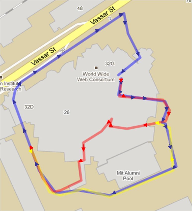
The system also was evaluated using a dataset taken in the
MIT campus in multiple sessions around of the Stata Center (b) Mixed (shadows)
building, with indoor and outdoor routes taken on July of
2010. The stereo images were collected with a BumbleBee2,
from PointGrey, with an 8cm baseline. We used 200 images
(512x384 px) uniformly distributed in time, from an indoor
session from April of 2010 to learn the weights for CRF-
Matching. In the fig. 4 we sketch the trajectories (using
Google Maps) and results. Both, our system and FAB-MAP
obtain similar results in precision and recall. The results of
our system spread more uniformly over the trajectory, see
Fig. 5. (c) Mixed (start-final)
IV. D ISCUSSION AND F UTURE WORK
We have presented a system that combines a bag-of-words
algorithm and conditional random fields to robustly solve
the place recognition problem with stereo cameras. We have
evaluated our place recognition system in public datasets
and in different environments (indoor, outdoor and mixed).
In all cases the system can attain 100% precision (no false
positives) with higher recall than the state of the art (less (d) Indoor (biggest loop)
false negatives), and detecting all (especially important) loop
Fig. 3. False negatives of FAB-MAP in the RAWSEEDS datasets. These
closure zones. No false positives mean that the environment scenes correspond to the biggest loop in the trajectories. In 3(a) the place
model will not be corrupted, and less false negatives mean was revisited 39 min later, and 36 min later in 3(c)
that it will be more precise. Our system also is more robust
in situations of perceptual aliasing.
In the context of place recognition over time, our system cases of periodical changes, such as times of day or seasons,
performs well in multi-day sessions using parameters learned incorporating a clock and calendar in the learning process
in different months, and this is also true of alternative sys- would allow to maintain several environment models and
tems such as FAB-MAP. The environment can also change select the most appropriate for a given moment of operation.
during the operation in the same session, see Fig. 3(a-c). Our One issue to consider is the stability of the extracted
algorithm is also able to detect places revisited at different descriptors in changing circumstances. In our case, SURF
times of day, while alternative systems sometimes reject them descriptors are useful when there is not much drift from its
in order to maintain high precision. invariance properties [14]. For example they are still useful
Several extensions are possible for operation in longer in the presence of outdoor seasonal changes [15], [16]. The
periods of time. The vocabulary for the BoW has shown same descriptors however do not seem useful to recognize
to be useful in different environments, which suggests that a places with totally different illuminations, e.g. an outdoor
rich vocabulary needs not be updated frequently. The learned scene from day to night.
parameters in the CRF stage can be re-learned in sliding When object locations change in a scene, we think that the
window mode depending on the duration of the mission. The MSTs still allows to properly encode the scene. The MST
system will then be able to adjust to changing conditions. In codifies mainly local consistency (features belonging to theFig. 5. Loops closure(green lines and stars) detected in the Stata Center multi-session dataset with FAB-MAP (top-left and bottom-middle) and our system
(top and bottom right). Different colours correspond to different sessions (blue, red and yellow). On the top, we show the query of the current frame vs.
the database with the frames already added. Ground truth (GT) is showed on bottom-left with magenta lines, on top with magenta circles.
thresholds as part of the learning stage would also make the
system more flexible.
ACKNOWLEDGEMENT
We thank Dorian Gálvez-López for his collaboration in the
hypothesis generation module of the place recognition sys-
tem and for releasing his hierarchical bag-of-word (DBow)
software library under an open source license available at
http://webdiis.unizar.es/˜dorian. We also thank John McDo-
nald for taking the datasets at the MIT campus with us.
R EFERENCES
[1] J. Sivic and A. Zisserman, “Video Google: A text retrieval approach
to object matching in videos,” in Proceedings of the International
Conference on Computer Vision, vol. 2, Oct. 2003, pp. 1470–1477.
[2] A. Angeli, D. Filliat, S. Doncieux, and J. Meyer, “A fast and
incremental method for loop-closure detection using bags of visual
words,” IEEE Transactions On Robotics, Special Issue on Visual
SLAM, vol. 24, pp. 1027–1037, 2008.
Fig. 4. Multisession experiment in the MIT campus. Different colours [3] M. Cummins and P. Newman, “FAB-MAP: Probabilistic Localization
correspond to different sessions. and Mapping in the Space of Appearance,” The International Journal
of Robotics Research, vol. 27, no. 6, pp. 647–665, 2008.
[4] ——, “Appearance-only SLAM at large scale with FAB-MAP
same object keep the same graph structure). Therefore, the 2.0,” The International Journal of Robotics Research, 2010.
inference process will still match features belonging to the [Online]. Available: http://ijr.sagepub.com/content/early/2010/11/11/
same object. Some cases of perceptual aliasing are possible 0278364910385483.abstract
[5] P. Piniés, L. M. Paz, D. Gálvez-López, and J. D. Tardós, “Ci-
if the same objects appear in different localizations, but these graph simultaneous localization and mapping for three-dimensional
cases will be much less frequent. reconstruction of large and complex environments using a multicamera
In our experiments, the β thresholds for acceptance of system,” Journal of Field Robotics, vol. 27, pp. 561–586, 2010.
[6] R. Paul and P. Newman, “FAB-MAP 3D: Topological mapping with
the CRF matching turned out to be clearly different for spatial and visual appearance,” in Proc. IEEE Int. Conf. Robotics and
indoor and for outdoors scenarios. These parameters will Automation, may. 2010, pp. 2649 –2656.
also depend on the velocity of motion, mainly due to the fact [7] C. Cadena, D. Gálvez-López, F. Ramos, J. Tardós, and J. Neira,
“Robust place recognition with stereo cameras,” in Proc. IEEE/RJS
that we use images from the previous second as reference Int. Conference on Intelligent Robots and Systems, Taipei, Taiwan,
in the comparisons. Incorporating the computation of these October 2010.[8] C. Cadena, J. McDonald, J. Leonard, and J. Neira, “Place recognition
using near and far visual information,” in 18th World Congress of the
International Federation of Automatic Control (IFAC), Milano, Italy,
August 2011.
[9] D. Nister and H. Stewenius, “Scalable recognition with a vocabulary
tree,” in Computer Vision and Pattern Recognition, 2006 IEEE Com-
puter Society Conference on, vol. 2, 2006, pp. 2161–2168.
[10] F. Ramos, D. Fox, and H. Durrant-Whyte, “CRF-Matching: Condi-
tional Random Fields for Feature-Based Scan Matching,” in Robotics:
Science and Systems (RSS), 2007.
[11] F. Ramos, M. W. Kadous, and D. Fox, “Learning to associate image
features with CRF-Matching,” in ISER, 2008, pp. 505–514.
[12] J. Lafferty, A. McCallum, and F. Pereira, “Conditional Random
Fields: Probabilistic models for segmenting and labeling sequence
data,” in Proc. 18th International Conf. on Machine Learning.
Morgan Kaufmann, San Francisco, CA, 2001, pp. 282–289. [Online].
Available: citeseer.ist.psu.edu/lafferty01conditional.html
[13] “RAWSEEDS FP6 Project,” http://www.rawseeds.org.
[14] P. Furgale and T. D. Barfoot, “Visual teach and repeat for long-range
rover autonomy,” Journal of Field Robotics, vol. 27, no. 5, pp. 534–
560, 2010. [Online]. Available: http://dx.doi.org/10.1002/rob.20342
[15] C. Valgren and A. J. Lilienthal, “Sift, surf & seasons: Appearance-
based long-term localization in outdoor environments,” Robotics and
Autonomous Systems, vol. 58, no. 2, pp. 149 – 156, 2010, selected
papers from the 2007 European Conference on Mobile Robots (ECMR
’07). [Online]. Available: http://www.sciencedirect.com/science/
article/B6V16-4X908T5-6/2/679a6246b247d1b8329211a2b9df49f4
[16] T. Krajnı́k, J. Faigl, V. Vonásek, K. Košnar, M. Kulich, and
L. Přeučil, “Simple yet stable bearing-only navigation,” Journal of
Field Robotics, vol. 27, pp. 511–533, September 2010. [Online].
Available: http://dx.doi.org/10.1002/rob.v27:5You can also read