POSITION ESTIMATION OF AUTONOMOUS UNDERWATER SENSORS USING THE VIRTUAL LONG BASELINE METHOD
←
→
Page content transcription
If your browser does not render page correctly, please read the page content below
International Journal of Wireless & Mobile Networks (IJWMN) Vol. 11, No. 2, April 2019

       POSITION ESTIMATION OF AUTONOMOUS
      UNDERWATER SENSORS USING THE VIRTUAL
              LONG BASELINE METHOD
  Alexander Dikarev, Stanislav Dmitriev, Vitaliy Kubkin and Andrey Vasilenko

        Underwater communication & navigation laboratory, LLC, Moscow, Russia

ABSTRACT
This article contains a description of a mathematical model of an acoustic system for positioning
autonomous underwater sensors using the virtual long base method, which can be used during the vessel’s
collection of information over the deployed underwater network of autonomous sensors (underwater
wireless sensors network), during the initial determination of the geographical position of the bottom long
baseline elements or search, including cooperative, with the use of a swarm of autonomous surface vehicles
(UASV) of emergency submerged objects equipped with an emergency beacon (for example, aircraft and
ships); The article provides a scheme of an experimental set of equipment, as well as a description of the
conducted field experiments and their results.

KEYWORDS

Underwater positioning system, VLBL, underwater wireless sensor network, emergency beacon positioning

1. INTRODUCTION

There is a wide range of tasks in which it is required to efficiently determine the geographical
location of submerged objects, while the external conditions impose restrictions on the use of a
long baseline navigation system (for example, time and complexity of deployment) and an
ultrashort navigation base (complex hydrological conditions, shallow water depth, high waves
etc.), lack of accuracy provided by USBL systems or any weight and size restrictions associated
with the applied vessel. Also, in some cases, the deployment of a long baseline (especially a
bottom one) is completely unjustified, for example, when quite rare (or single) measurements of
the underwater object’s position are required, or in case of a search (for example, accidentally
submerged objects — ships or aircraft[1][2]) in a fairly wide area, where it is impossible to install
a long baseline system of the required dimensions. Particularly noteworthy is the positioning of
the nodes of Underwater wireless network of autonomous sensors UWSN[3][4] which often
require only a rare or even a one-time estimation of their location. In more detail, the problems of
localization of nodes of wireless underwater sensor networks are discussed in [5][6][7].

Problems that discussed above can be successfully solved using a virtual long baseline approach
[8][9][10]. The key point here is the immobility of the objects being positioned, which makes it
possible to measure distances from different positions on the surface (in the case of the TOA
method[6][11]) or pseudo ranges (in the case of the TDOA method [12][13][14]). In both cases,
clocks of the requesting system and the desired object are not synchronized. The second option
provides the possibility of a cooperative search for an underwater object by a swarm of

DOI: 10.5121/ijwmn.2019.11202                                                                           13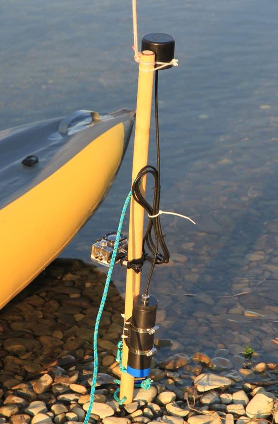
International Journal of Wireless & Mobile Networks (IJWMN) Vol. 11, No. 2, April 2019
autonomous vehicles [15][16]: an object periodically emitting a navigation signal, allows
simultaneous reception on an unlimited number of surface receivers, thereby providing coverage
for a theoretically arbitrarily large search area.
Let us consider in more detail the model of the system described in this article.
2. SYSTEM MODEL
The following formatting rules must be followed strictly. Assume there is a submerged stationary
object, whose position, expressed in its coordinates xo, yo, zo, has to be estimated. The object is
equipped with a hydroacoustic responder beacon, transmitting pressure and temperature sensor
readings on request from outside. In general, distance do (slant range) to it is estimated on the
requesting system as:
d o = (Ta − Tt − Td ) / 2
(1)
Where Ta - the time of arrival of the response from the responder by the clock of the requesting
system, Tt - the time of the beginning of the request signal radiation by the clock of the requesting
system, Td - constant response delay.
If the requesting system moves, and at different points in time measures the distance to the
responder, then a set doi of measurements are formed, matching the locations of the requesting
system xri, yri, zri.
The solution to the problem of estimating the location of the desired object for a given set of
measurements in general form consists in finding the global minimum of the residual function ε:
N
(
( x, y, z ) = ( x − xri ) 2 + ( y − yri ) 2 + ( z − zri ) 2 − d oi
i =1
)
2
(2)
However, the sequential set of points obtained in the process of moving the requesting system is,
firstly, redundant, and secondly, it is a deliberately disadvantageous arrangement of virtual
reference points: in a line and/or group on one side of the desired object with a distance between
points less than to the desired object. All of this leads to a “blurring” of the desired minimum of
the function ε and/or the formation of false minima that do not correspond to the true position of
the desired object. This case is illustrated in Figure 1.
Fig. 1 - False minimum with an unsuccessful selection of base points
14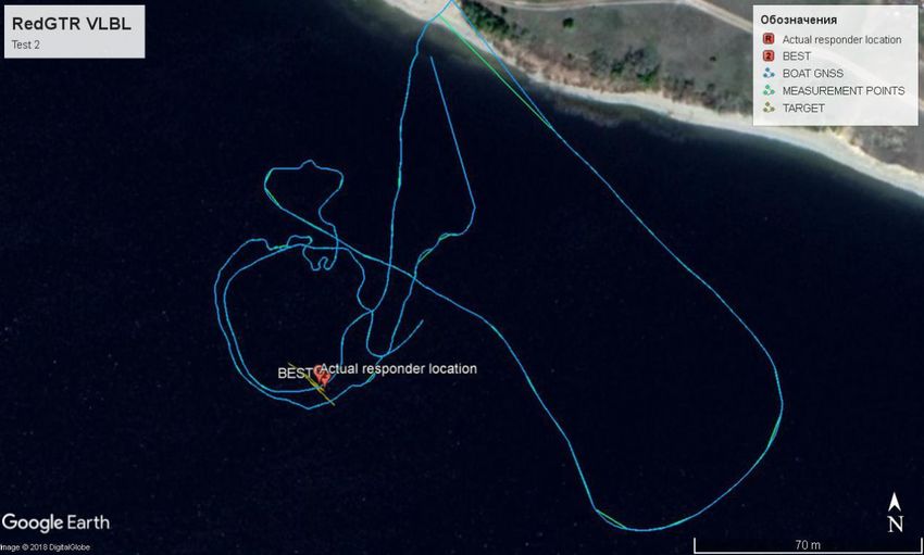
International Journal of Wireless & Mobile Networks (IJWMN) Vol. 11, No. 2, April 2019
Consequently, the problem of estimating the location is now divided into two subproblems: the
selection of the optimal base - the selection of the optimal set of measurements to solve the
position estimation problem and the actual solution of the position estimation problem.
Since, in general, the location of the desired object is unknown even approximately, there is no
way to pre-select the optimal trajectory of the requesting system and there are no criteria for
selecting the optimal navigation base.
One possible option of the initial base selection may be such a heuristic approach, where the point
at which it is supposed to look for a solution selected from the conditions to maximize diversity
angular directions αmi from some point M(xm, ym, zm), as the initial stage, it is proposed to choose
the geometric center of the entire set of measurements doi. In this case, it becomes possible to at
least get a flat base pattern (rather than a line), on the basis of which one can get the first
approximation of the position of the desired object, which one then choose as a point M, and
carry out a selection of base points according to the condition of ensuring the maximum variety of
angular directions from this point, which in many cases will allow obtaining a figure of the
navigation baseline described around the desired object. This strategy is illustrated in Figure 2.
Fig. 2 - Formation of the navigation base from the entire set of measurements, the number of elements of
the base is 6
In Figure 2, the rectangles indicate the set of points Ai, representing the trajectory of the
requesting system, the circles are points selected as elements of the virtual navigation base.
The angular direction αMAi from the selected point M(xm, ym, zm) to some point Ai(xri, yri, zri), at
which the distance was measured is determined from a simple trigonometric equation:
sin( M − Ai ) cos Ai
MAi = arctan
cosM sin Ai − sin M cos Ai cos( Ai − M ) (3)
15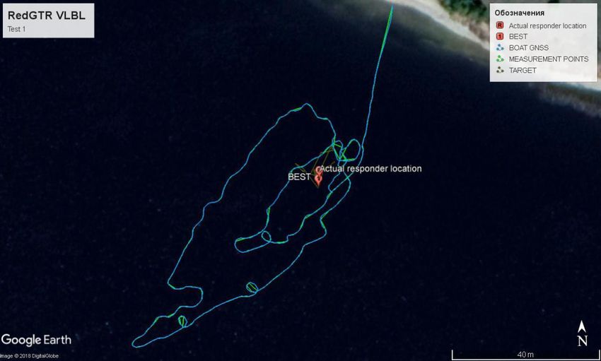
International Journal of Wireless & Mobile Networks (IJWMN) Vol. 11, No. 2, April 2019
where λM and φM - longitude and latitude of the selected point M, λAi and φAi - longitude and
latitude of point Ai respectively.
Further, to select points-virtual elements of the navigation base, the following steps are performed:
- the whole set of measurements is sorted by the angular direction αMAi, and there are two such
neighboring points Ai and Ai+1, for which the absolute difference modulus Δα will be the
maximum of the entire set. These points can be considered the boundaries of the entire available
angular range. This operation must be performed because, in the general case, the angular
directions αMAi do not necessarily evenly fill the entire circle; At this stage, the starting αs and the
ending αe angles of the available angular range are determined, the angular range αr itself:
r = 2 − ( e − s ) (4)
- At this stage, the desired angular directions are determined in which it is necessary to install the
virtual elements of the navigation base. The desired angular gap αΔ between the elements is
defined as:
= r /( N B −1) (5)
Where NB - the required number of virtual elements of the navigation base.
For the case where Δαmax is lower than αΔ, the last decreases accordingly to (6), otherwise it may
turn out that measurements with angular directions αs and αe will be selected as base elements,
while the angular distance between them will be less than αΔ, which, in turn, for small NB will
result in an uneven arrangement of the base elements in the angular direction.
( − max )( N B − 1)
= −
( N B − 2) N B (6)
- The desired angular directions αBi are determined at this stage.
Bi = s + i , i 0..N B − 1 (7)
- at the final stage, such NB measurements are selected from the entire set, in which the angular
directions are closest by value to the desired ones.
Now, the solution of problem (2) is possible by one of the optimization methods. However, as it
is often the case, and as mentioned above, there is no guarantee in selecting the optimal base
configuration, and the residual function may have false minimums. To solve this problem, one
can apply the following approach, which is a rough estimation of the position of the global
minimum using the one-dimensional optimization method. It is worth mentioning that this
approach is applicable only in the case of the distance measuring method when the distances to
the desired object are measured directly.
So, since the distance to the virtual elements of the navigation base and the depth of the
transceiver of the requesting system and the desired object are known, the desired object is
located on circles in which centers there are virtual base points. The x and y coordinates of the
desired object, in this case, are expressed through the angle β:
x = xrn + d rn cos
y = yrn + d rn sin
(8)
16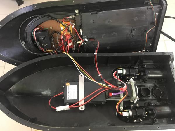
International Journal of Wireless & Mobile Networks (IJWMN) Vol. 11, No. 2, April 2019

xrn, yrn and drn - the coordinates of the nearest base point and the projection of the slant range to it,
respectively. Having performed a complete search over β in the range from 0 to 2π with a certain
step (in this work, a search with a step of 10 degrees and then a search with a step of 1 degree in
the range of +/- 10 degrees from the previous minimum position are used), one can obtain an
approximate position of the global minimum of the function (2), which then will be used as the
initial one for solving a two-dimensional problem.

Figure 3 shows a comparison of the effectiveness (number of iterations) of solving the problem of
estimating the location of the desired object of random data with and without the application of
preliminary one-dimensional optimization.

Figure 4a and b show the distribution of errors (distances from the actual position of the object to
the calculated one) on the same random sample, for the variant without preliminary optimization
and with such. A random error with a uniform distribution and an amplitude of 1 meter was
injected into the distance measurements.

  Fig. 3 - The number of iterations to obtain convergence without the use of preliminary one-dimensional
                  optimization and with such. Sample size 256, number of base stations 4

The two-dimensional problem was solved using the Nelder – Mead method[17], and the value of
the residual function (2) at the output of one-dimensional optimization was used to specify the
initial size of the simplex.

As can be seen from Figure 3, a preliminary one-dimensional optimization, firstly, almost
eliminates falling into a false minimum, and secondly, significantly reduces the number of
iterations required to achieve a solution with satisfactory accuracy. In this case, the one-
dimensional optimization procedure has a fixed execution time, which is also important for real-
time systems.

                                                                                                       17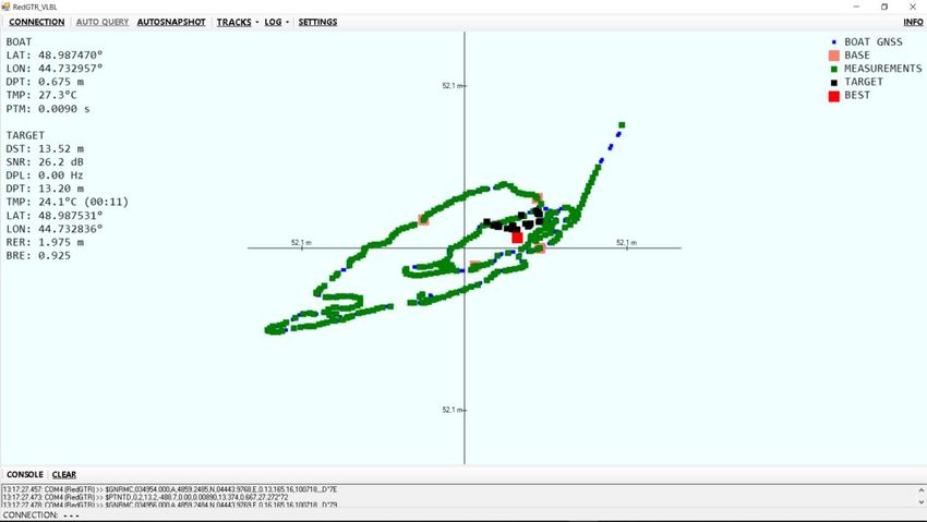
International Journal of Wireless & Mobile Networks (IJWMN) Vol. 11, No. 2, April 2019

                                                          а)

                                                          b)
         Fig.4 - the distribution of the error of estimating the location of the desired object without the use
          of one-dimensional preliminary optimization (a) and with the use of such (b). Sample size 256,
                                                number of base stations 4

From histograms in fig. 4a) by significant errors of hundreds of meters it is clear that the search
went to a false minimum, and in fact, this led to an absolutely wrong result, at the same time
according to the histogram in fig. 4b) when using preliminary one-dimensional optimization, this
situation is not observed, and the positioning error has a value comparable to the artificially
introduced error (~ 1 m).

3. EXPERIMENTAL SETUP

A     set    of    experimental   equipment      consists    of    the     following     parts:
The desired underwater object - the responder beacon, which was used as a standalone
RedGTR[18] modem in an autonomous version with a built-in pressure sensor. A modem with a
battery pack was mounted on a pole with a load and float, providing a vertical position in the
submerged state. The modem, among other things, supports the transmission of readings from the
                                                                                                             18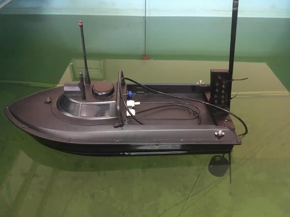
International Journal of Wireless & Mobile Networks (IJWMN) Vol. 11, No. 2, April 2019

built-in depth and temperature sensor, has a fixed signal length (400 ms), allows operation in the
request-response mode, and supports a simple NMEA0183-like interface protocol. It also has
small dimensions, weight, and provides communication range of up to 8000 meters. A
submersible stand with a modem is shown in Figure 5.

                           Fig. 5 - Submersible stand with a RedGTR modem

The requesting system consists of a small radio-controlled vessel equipped with a GPS/
GLONASS receiver, a motherboard based on the STM32F429 processor[19], a RedGTR modem,
and a digital radio module[20]. Appearance and internals of the vessel are shown in the photo in
Fig. 6

                      a)                                                     b)
                            Fig. 6 - Appearance (b) and internals (a) of a test vessel

                                                                                                19
International Journal of Wireless & Mobile Networks (IJWMN) Vol. 11, No. 2, April 2019
The scheme of the requesting system is shown in Figure 7.
Fig. 7 - Scheme of the requesting system
The experimental test consisted of the following steps:
- alternately at the bottom of the reservoir in two places there was a submersible stand;
- the vessel described above, which was controlled by radio from the shore, moved along a free
trajectory through the reservoir. On command by a specially developed software, the source code
of which is freely available [21], requests were periodically initiated from a modem located on the
ship to a modem located on a submersible stand. At the same time, the ship’s computational
module transmitted its GPS location data and retransmitted the beacon response over the radio;
The frequency of requests was limited only by the modems themselves and amounted to about 1
time in 2 seconds. The time of one request-response transaction is made up of double the duration
of the modem signal Ts = 400 ms, the fixed response delay Td = 800 ms, and the double
propagation time of the signal depending on the slant range between the transponder and the
inquiring system.
The speed of the vessel varied from 0 to 1 m/s. The experiments were carried out in June 2018 at
the mouth of the Pichuga River, at the place of its inflow into the Volgograd water reservoir
(48°59’12.86’’N 44°43’52.24’’E). The depths in the places of the experiments varied from 2 to
20 meters, the bottom is sandy and rocky, the width of the river at the place of work is 350 meters.
In the course of the work, the following data were recorded:
- the initial position of the responders before diving using a GPS/GLONASS receiver based on a
Quectel L76[22];
20International Journal of Wireless & Mobile Networks (IJWMN) Vol. 11, No. 2, April 2019
- the position of the vessel according to the built-in GPS/GLONASS receiver;
- the depth of the modem of the requesting system;
- water temperature according to the data of the modem’s built-in sensor of the requesting system;
- temperature according to the built-in modem sensor on the desired object;
- depth according to the built-in modem’s sensor on the desired object;
- distance (slant range) from the requesting system to the desired object with reference to the
geographical location of the requesting system, where the measurement was made;
- the calculated geographic location of the desired object;
4. EXPERIMENTAL RESULTS
The main results of this work are the tracks stored in the Google KML format, containing the
following data:
- a track movement of the requesting system (vessel), according to the onboard GNSS;
- a track containing the points at which distance measurements were made to the desired object;
- a track containing points obtained by calculating the coordinates of the desired object, according
to the procedure described in this paper;
- the marked point that has a minimal radial error (the value of the function ε according to (2));
- the marked point at which the respondent was actually submerged;
Tracks containing data from two experiments are available on GitHub [23] [24] along with the
source code of the application [21].
The distance of the modem of the requesting system from the surface of the water varied from 0.5
to 0.75 meters.
The depths of the respondents were 13.2 and 16.5 meters for the first and second experiments,
respectively.
Fig. 8 shows a screenshot of the main application window in the process of work (the first
experiment).
Fig. 8 - Screenshot of the main application window
21International Journal of Wireless & Mobile Networks (IJWMN) Vol. 11, No. 2, April 2019
As can be seen from Figure 8, the described system allows not only to monitor the location of the
object being searched for but also to correct the vessel's heading, determine the depth of the
object being searched, as well as the water temperature using its built-in sensor. The RER and
BRE fields correspond to the current and best values of the residual function (2).
According to the calculated positions of the object, the deviation from the real position obtained
using GNSS just before the submersion is in the range of 2-2.5 meters in both experiments, which
is comparable with the accuracy of the used GNSS modules [22].
A general view of the tracks obtained in this work is presented in Fig. 9 and 10.
Fig.9 - Screenshot of the GoogleEarth application window with tracks obtained during the first experiment
Fig.10 - Screenshot of the GoogleEarth application window with the tracks obtained during the
second experiment
22International Journal of Wireless & Mobile Networks (IJWMN) Vol. 11, No. 2, April 2019
5. CONCLUSION
The results of mathematical modeling and field experiments confirm:
- the adequacy of the system model to real conditions;
- the ability to ensure the localization of stationary submerged objects, equipped with responders
using mobile surface uninhabited vehicles; If it is necessary to localize several underwater objects
at the same time (for example, nodes of an underwater wireless network of sensors), the selected
scheme as a whole can be saved with the only exception that all objects will be polled in turn,
which will correspondingly increase the localization time;
- the accuracy of the location estimation of the underwater objects in the experiments performed
is comparable to the declared accuracy of the used GNSS receivers;
- the need to apply the proposed method of pre-refinement of the location.
Further studies in this area are planned using the TDOA method, which will allow the use of a
much simpler device mounted on an underwater object, so-called pinger that does not contain a
receiving hydroacoustic unit; At the same time, this scheme will allow excluding the transmitting
hydroacoustic unit from the system that performs the search, and also allows, as already
mentioned, to apply cooperative search using a swarm of surface vehicles.
REFERENCES
[1] BEA – Bureau of Enquiry and Analysis for Civil Aviation Safety, “Final report on the accident on 1st
June 2009 to the Airbus A330-203”, June 2009, pp. 1–223, 2012
[2] Barmak, Rafael & L S C De Oliveira, André & São Thiago, Pedro & V R Lopes, Marco &
Cernicchiaro, Geraldo & dos Santos, Francisco. (2017). Underwater Locator Beacon signal
propagation on tropical waters. 10.1109/RIOAcoustics.2017.8349738.
[3] Akyildiz, I.F. and D. Pompili, 2005. Underwater Acoustic sensor Networks: Research Challenges A
survey, pp: 257-279
[4] Manjula R.B., Sunilkumar S. Manvi, 2011. Issues in Underwater Acoustic Sensor Networks,
International Journal of Computer and Electrical Engineering, Vol.3, No. 1, February, 2011, pp.101-
102
[5] Long Cheng, Chengdong Wu, Yunzhou Zhang, Hao Wu,Mengxin Li, Carsten Maple., A Survey of
Localization in Wireless Sensor Network. Hindawi Publishing Corporation International Journal of
Distributed Sensor Networks Volume 2012, Article ID 962523, 12 pages doi:10.1155/2012/96252
[6] Ravindra S., Jagadeesha S. N., Time of arrival based localisation in wireless sensor networks: a linear
approach. Signal & Image Processing : An International Journal (SIPIJ) Vol.4, No.4, August 2013
[7] Chien-Chi Kao, Yi-Shan Lin, Geng-De Wu and Chun-Ju Huang, A Comprehensive Study on the
Internet of Underwater Things: Applications, Challenges, and Channel Models. Sensors 2017, 17,
1477, doi:10.3390/s17071477
[8] LaPointe, Cara E. G.. “Virtual Long Baseline ( VLBL ) Autonomous Underwater Vehicle Navigation
Using a Single Transponder.” (2006).
23International Journal of Wireless & Mobile Networks (IJWMN) Vol. 11, No. 2, April 2019
[9] Sarah E Webster, Ryan M Eustice, Hanumant Singh, and Louis L Whitcomb, Advances in single-
beacon one-way-travel-time acoustic navigation for underwater vehicles. The International Journal of
Robotics Research Vol 31, Issue 8, pp. 935 – 950
[10] JoÃo Saúde, Antonio Pedro Aguiar, Single Beacon Acoustic Navigation for an AUV in the presence
of unknown ocean currents, IFAC Proceedings Volumes, Vol. 42, Issue 18, 2009, pp. 298-303, ISSN
1474-6670, ISBN 9783902661517, https://doi.org/10.3182/20090916-3-BR-3001.0057.
[11] K. W. Cheung, H.C. So, W.-K. Ma and Y.T.Chan, (2004) “Least squares algorithms for time-of-
arrival based mobile location,” IEEE Transactions on Signal Processing, vol.52, no.4, pp.1121-1128.
[12] Abdulmalik S. Yaro, Muazu J. Musa, Salisu Sani, Abdulrazaq Abdulaziz, 3D Position Estimation
Performance Evaluation of a Hybrid Two Reference TOA/TDOA Multilateration System Using
Minimum Configuration, International Journal of Traffic and Transportation Engineering 2016, 5(4):
96-102
[13] Fatima S. Al Harbi, Hermann J. Helgert. An Improved Chan-Ho Location Algorithm for TDOA
Subscriber Position Estimation, IJCSNS International Journal of Computer Science and Network
Security, VOL.10 No.9, September 2010
[14] Y. T. Chan, and K. C. Ho, “A simple and efficient estimator for hyperbolic location,” Signal
Processing, IEEE Transactions on, vol. 42, no. 8, pp. 1905-1915, 1994.
[15] Wei Zhao, Zhenmin Tang, Yuwang Yang, Lei Wang, and Shaohua Lan, “Cooperative Search and
Rescue with Artificial Fishes Based on Fish-Swarm Algorithm for Underwater Wireless Sensor
Networks,” The Scientific World Journal, vol. 2014, Article ID 145306, 10 pages, 2014.
https://doi.org/10.1155/2014/145306.
[16] B. T. Champion and M. A. Joordens, "Underwater swarm robotics review," 2015 10th System of
Systems Engineering Conference (SoSE), San Antonio, TX, 2015, pp. 111-116. doi:
10.1109/SYSOSE.2015.7151953
[17] J. A. Nelder, R. Mead; A Simplex Method for Function Minimization, The Computer Journal, Volume
7, Issue 4, 1 January 1965, Pages 308–313, https://doi.org/10.1093/comjnl/7.4.308
[18] RedGTR underwater acoustic modem specification,
https://github.com/ucnl/Docs/blob/master/EN/Modems/RedGTR/RedGTR_Specification_en.pdf,
retrieved on 10 Jan 2019
[19] STM32F429 Cortex-M4 Processor product datasheet
www.st.com/resource/en/datasheet/stm32f427vg.pdf, retrieved on 18 Aug 2018
[20] DRF7020D27 27 dBm ISM RF Transceiver Module, Product datasheet,
http://dorji.com/docs/data/DRF7020D27.pdf, retrieved on 18 Aug 2018
[21] https://github.com/ucnl/RedGTR_VLBL, retrieved on 18 Aug 2018
[22] Quectel L76 Compact GNSS Modules, Product datasheet,
https://www.quectel.com/UploadFile/Product/Quectel_L76_GNSS_Specification_V1.4.pdf
[23] https://github.com/ucnl/RedGTR_VLBL/blob/master/Samples/Tracks/10-07
2018_RedGTR_VLBL_Test_1.kml, retrieved on 18 Aug 2018
24International Journal of Wireless & Mobile Networks (IJWMN) Vol. 11, No. 2, April 2019
[24] https://github.com/ucnl/RedGTR_VLBL/blob/master/Samples/Tracks/10-07-
2018_RedGTR_VLBL_Test_2.kml, retrieved on 18 Aug 2018
Authors
Alexander Dikarev
received his M.Eng in Launching equipment of rockets and cosmic apparatus from
Volgograd Technical State University, Russia. He has 10 years experience in
underwater acoustic comm unication and navigation system design and development:
in Research Insitute of Hydroacoustic Communications (Volgograd, Russia), The
University Of Manchester (UK), now he is R&D Director in Underwater
communication & Navigation laboratory (Moscow, Russia)
Stanislav Dmitriev
received his M.Sc in Radiophysics in Volgograd State University, Russia. He has 10
years of experience in Underwater Acoustic communication & navigation system
design & development: in Research Insitute of Hydroacoustic Communications
(Volgograd, Russia), now he is Engineering Director in Underwater Communication
& Navigation laboratory (Moscow, Russia)
Vitaliy Kubkin
received his M.Eng in Volgograd Technical State University, Russia. He has 10
years of experience in Underwater Acoustic communication & navigation system
design & development: in Research Insitute of Hydroacoustic Communications
(Volgograd, Russia), now he is Senior Researcher in Underwater Communication &
Navigation laboratory (Moscow, Russia)
Andrey Vasilenko
Received his M.Sc in Radiophysics in Volgograd State University, Russia. He has
more than 15 years of experience in Underwater Acoustic communication &
navigation system design & development: in Research Insitute of Hydroacoustic
Communications (Volgograd, Russia), now he is Chief Electronics Engineer in
Underwater Communication & Navigation laboratory (Moscow, Russia)
25You can also read