Simultaneous Load Disturbance Estimation and Speed Control for Permanent Magnet Synchronous Motors in Full Speed Range - MDPI
←
→
Page content transcription
If your browser does not render page correctly, please read the page content below
applied
           sciences
Article
Simultaneous Load Disturbance Estimation and
Speed Control for Permanent Magnet Synchronous
Motors in Full Speed Range
Yingming Tian 1,2 , Yi Chai 1, * and Li Feng 3
 1    College of Automation, Chongqing University, Chongqing 400044, China; tianyingming@cqcy.com
 2    Chongqing Chuanyi Automation Co., Ltd., Chongqing 401121, China
 3    College of Traffic and Transportation, Chongqing Jiaotong University, Chongqing 400074, China;
      fengli@cqjtu.edu.cn
 *    Correspondence: chaiyi@cqu.edu.cn

 Received: 18 November 2020; Accepted: 15 December 2020; Published: 16 December 2020

 Abstract: Permanent magnet synchronous motors (PMSM), which are with the advantages of high
 torque-to-weight ratio and high efficiency, are widely applied in modern industrial systems. However,
 existing approaches may fail to accurately track the speed trajectory because of the load disturbances.
 This paper proposes an equivalent and combined control strategy to mitigate the slow time-varying
 load disturbances and decrease the overshoot for PMSM in full speed range. First, a state observer
 is proposed to reconstruct the current variables and speed state in the d-q axis. Hence, one can get
 the speed and position information without the sensors. Then, the disturbance and the load are
 estimated by the estimating law. Thus, it can reduce the effect of load and disturbances. Further,
 the PD control is introduced to weaken the overshoot. As a result, the speed trajectory can be more
 effectively hold both in high speed and low speed. Finally, numerical examples are presented to
 demonstrate the validity and effectiveness of the proposed estimation scheme and its robustness
 under different conditions.

 Keywords: state observer-based control; PD control; permanent magnet synchronous motors (PMSM);
 speed control

1. Introduction
     Permanent magnet synchronous motors (PMSM) have been widely used in the fields of
electric vehicle drive system, robot, aerospace, intelligent manufacture, and other fields because
of the advantages of excellent efficiency, high power density, low inertia, high torque-current ratio,
no excitation loss, et al. [1]. In order to ensure the smooth running of the motor, it is very important
to adopt efficient and stable control strategies for each part of the three-phase permanent magnet
synchronous motor system, such as speed control [2], current control [3], and pulse width modulation [4].
Besides, sensor-less control also needs observer strategy or other control methods [5]. Among them,
speed control is particularly important.
     The control of current loop can be simply divided into current control in static coordinate system
and current control in synchronous rotating coordinate system. For the current control in synchronous
rotation coordinates, hysteresis current control and PI current control are commonly used at present.
Hysteresis current control can meet the requirements of motor operation, but the electromagnetic torque
fluctuates greatly during the whole starting process, and PI regulator has good dynamic performance
and anti-disturbance ability, which can meet the needs of actual motor control performance [6].
The pulse width demodulation technology of three-phase voltage source inverter mainly includes

Appl. Sci. 2020, 10, 9006; doi:10.3390/app10249006                              www.mdpi.com/journal/applsci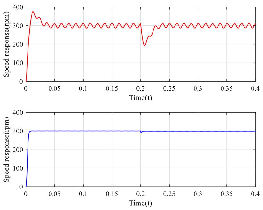
Appl. Sci. 2020, 10, 9006                                                                          2 of 13

two-level space vector pulse width modulation (SVPWM) and sinusoidal pulse width modulation
(SPWM). SVPWM has better harmonic elimination effect and torque ripple resistance than SPWM [7].
      In recent years, many control technologies are used in the research of speed control for PMSM,
which can be divided into linear control and nonlinear control [8]. As is known to us all, many linear
control methods based on transfer functions (the most popular one is PI control [9]) are sensitive to the
system model accuracy, which is highly susceptible to external disturbances and internal parameter
mismatch. Therefore, many scholars draw attention on nonlinear control design for PMSM, such as
robust control [10], adaptive control [11], and sliding mode control [12].
      Among these speed control strategies for PMSM, sliding mode control with the merits of simple
structure and fast response has become one of the most popular methods. In reference [13], a nonlinear
speed-control algorithm for the PMSM control systems using sliding-mode control (SMC) is proposed
to optimize the dynamic performance of speed regulation system. In which, the new sliding-mode
reaching law (NSMRL) using the system state variable and the power term of sliding surface function
can be expressed in two different forms during the reaching. This method can not only effectively
suppress the inherent chattering, but also increases the velocity of the system state reaching to the
sliding-mode surface. A new adaptive terminal sliding mode reaching law (ATSMRL) is proposed
with continuous fast terminal sliding mode control (CFTSMC) in reference [14]. It aims to enhance the
speed control performance of the permanent magnet synchronous motor (PMSM) with internal and
external disturbances. In reference [15], a novel sliding mode control (NSMC) strategy is developed
to improve the robustness, disturbance rejection, and dynamic response performance of permanent
magnet synchronous motor (PMSM) speed servo system. The integral of speed error is introduced into
sliding mode surface to avoid the requirements of acceleration signal and reduce the steady-state error
of the system. It can be found in the existing literature that many scholars focus on the design of new
sliding mode reaching law and novel sliding mode surface. One cannot deny that these literatures have
achieved good control performance. However, sometimes it is hard to know how to get a new reaching
law or a new sliding mode surface, that is, it requires more professional and profound knowledge of
sliding-mode control theories.
      Nowadays, to get better performance, the integration of control categories with other methods
have been a hotspot. The authors propose a speed observer based on back-stepping and sliding mode
for low-speed operation in [16]. The reference [17] develops a low-order adaptive instantaneous speed
estimator (AISE) and a self-tuning control strategy to improve the speed control performance in a
wide speed range with unknown inertia parameters. In reference [10], a model predictive direct speed
control (MPDSC) method is proposed to get a good anti-disturbance ability for PMSM. It depends
both on full parameter disturbances and load torque observer and the precise mathematical model
parameters are not needed. Actually, these methods combine the advantages of various algorithms so
as to get good performance.
      This paper develops a sliding mode control strategy associated with a load disturbance estimator
to enhance the dynamic performance of PMSM in full speed range. The proposed estimator can
reconstruct the disturbance in load caused by the variation of load environments. Then, PD control
is employed to decrease the overshoot. Finally, the speed tracking performance can be improved
by designing an equivalent control law. Further, numerical examples are proposed to verify the
effectiveness of the presented method under both high speed and low speed.
      The rest of this paper is organized as follows. Section 2 describes the model of PMSM, in which,
the disturbance and uncertainties are discussed and modeled. An estimator and control strategies
are designed in Section 3. Then the main theoretical results are shown in Section 4. Finally, Section 5
summarizes the innovations of this thesis and makes a prospect of this paper.

2. Materials and Methods
    In this section, PMSM mathematical model is constructed to support the design of control strategy.
Disturbance and uncertainties are modeled to clarify its impact on the system. Hence, one can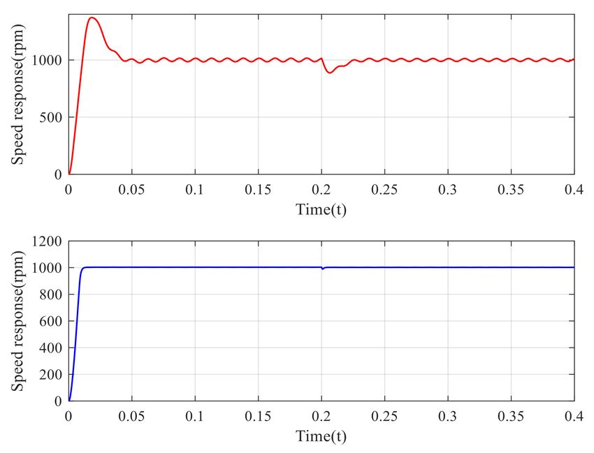
Appl. Sci. 2020, 10, 9006 3 of 13
understand how disturbance and uncertainties affect the performance of the PMSM system. Then,
the estimator and controller are designed to deal with the corresponding problems and achieve speed
regulation goals.
2.1. PMSM Mathematical Model
PMSM plays an increasingly important role in the speed regulation system because of its significant
advantages in structure, efficiency, and so on compared with other types of motors. In existing literatures,
all the PMSM mathematical model are based on the conventional assumption [15]. In order to improve
the effectiveness of the speed controller, this paper considers the mathematical model in the d-q
synchronous rotating reference. The stator’s voltage equation is shown as follows.
d
ψd − ωe ψq
(
ud = Rid + dt
(1)
uq = Riq + dt ψq + ωe ψd
d
in which, subscript d and q refer to the d-component and q-component. u, i, and ψ represent the stator’s
voltage, stator’s current, and stator’s flux, respectively. Then ωe is the electrical angular velocity and R
is the stator resistor.
For surface-mounted PMSM, it can be obtained that stator inductor Ls = Ld = Lq . The following
mathematical model with the assumption that B = 0 is as following:
did
dt = Ls −Rid + pn Ls ωm iq + ud
1
diq
dt = Ls −Riq − pn Ls ωmid − pn ψ f ωm
1
+ uq (2)
3pn ψ f
dωm 1
dt = J −TL + 2 iq
in which, ψ f is the flux of magnet, pn is the pole pairs of PMSM, ωm is the mechanical angular velocity,
J is the inertia, B is the friction coefficient, and TL is the load torque.
Based on the characters of PMSM, one can get that ωm , id , and iq are variables and bounded. Thus,
the nonlinear term in (2) is bounded and the varying range is determined by the value of mentioned
parameters above.
As is known to all scholars, the controller can achieve better performance according to using rotor
field orientation control (id = 0) strategy. Then, the mathematical model in Equation (2) can be written
as follows. di
q
dt = L1s −Riq − pn ψ f ωm + uq
(3)
dωm = 1 −T + 3pn ψ f i
dt J L 2 q
Therefore, the complex nonlinear mathematical model function is simplified and linearized.
2.2. System Model for Disturbance Estimator Design
It can be easily found that equation is obtained by the common assumptions. The rotor’s magnetic
field is sinusoidal in the air gap space. The saturation of stator core, core Eddy current, hysteresis
loss, and damping of rotor windings are ignored. It is also assumed that the magnetic circuit is linear.
However, these factors will affect the performance of PMSM in the actual operating environment.
Simultaneously, the nonlinear terms in system (2) also deteriorate the operating effects. Linearizing the
nonlinear system with linear equation will make the research relatively simple, but it cannot completely
reflect the complicated actual situation, so the accuracy of the calculation result is relatively low [18].
In this subsection,h we will discuss
i the effects by modeling and quantifying these factors.
Define that xT = iq ωm , y = xT , u = uq , then one can get that
.
x = Ax + Bu + Eξ
(4)
y = CxAppl. Sci. 2020, 10, 9006 4 of 13
h iT h i
in which, the parameters can be obtained by Equation (6) as A = A1 A2 ,A1 = L1s −R −pn ψ f ,
" #
1 3pn ψ f
h i h
1
iT h
1 T
i 1 0
A2 = J 2 0 , B = Ls 0 , E = 0 − J ,C= , ξ = TL .
0 1
Then, it can be assumed that the influence of fore-mentioned factors, including saturation of
stator core, hysteresis loss, and so on, can be quantified in the system load disturbances. The details of
considering the factors are as follows.
.
x = Ax + Bu + E(ξ + δ) (5)
where δ represents the load disturbances. Define that d = ξ + δ. One can get that
.
x = Ax + Bu + Ed (6)
Based on the model (6), the observer and estimator can be constructed to get the load, disturbance
value, and the estimation of x. It will be further discussed in the next section.
In practice, the dynamic change of load will cause load disturbance, and the output speed of
motor will also shake, which greatly affects the motion accuracy and working stability of PMSM drive
system [19]. How to suppress this load disturbance caused by load change is what this paper is doing.
2.3. System Model Design for Combined Controller
To get better control performance, we redefined the state variables and constructed another system
function in this subsection.
First, the state variable is defined as:
z1 = ωre f − ωm
. . (7)
z2 = z1 = −ωm
in which, ωre f is the reference speed of PMSM, usually, it is set as a constant value. Hence, one can
get that
3pn ψ f
. .
z = − ω = 1
T − i
1 m L q
J 2
(8)
z. = −ω
.. 3pn ψ f .
2 m = − 2J iq
Then, one can obtain the system as follows.
" . # " #" # " #
z1 0 1 z1 0
. = + u0 (9)
z2 0 0 z2 −D
. 3pn ψ f
where u0 = iq and D = 2J .
Conventionally, sliding surface and reaching law are designed to construct the control strategy in
order to achieve good performance. But abundant experiences and knowledge are needed to improve
them. To solve the mentioned problems above, this paper proposes a novel combined control approach
based on the principle of equivalent control.
3. Main Results
This section may be divided by subheadings. It should provide a concise and precise description
of the experimental results, their interpretation, as well as the experimental conclusions that can
be drawn.
3.1. Design of the Combined Estimator
In speed regulation of PMSM, model simplification and operating environments may cause the
parameter uncertainties and load disturbances. Hence, the dynamic and steady-state performanceAppl. Sci. 2020, 10, 9006 5 of 13
of PMSM will be reduced. In this paper, a compensational estimator is presented to reconstruct the
modeled disturbance signal, which contains the influence of both parameter uncertainties and load
disturbance. They can be used in controller design to improve the capability for anti-jamming.
Based on the system (5), state observer is proposed as follows.
.
x̂ = Ax̂ + Bu + Edˆ + L( ŷ − y)
(10)
ŷ = Cx̂
h iT
where x̂ and dˆ are the estimation of x and d. L = L1 L2 represents the observer gain matrix.
The compensational estimator is presented as Equation (11) if d is a slow time-varying signal.
.
dˆ = K(x̂ − x) (11)
in which, K is the estimator gain matrix, and the parameters in K are positive. Then it is followed by
the stability analysis of the proposed method.
Lemma 1. Based on system (9) and the estimator (11), one can get that the observer (10) and estimator (11) can
achieve good performance if the following inequality holds [20].
(A − LC) ≤ 0 (12)
Hence, one can get that the proposed method can achieve stable convergence.
Proof 1: The Lyapunov function is defined as
E ˜2 1 2
V= d + x̃ (13)
2K 2
where d˜ = d − d,ˆ x̃ = x − x̂. The derivative can be written as
. . .
V = KEd˜d˜ + x̃x̃
. . h i
= d˜ d − dˆ + x̃ Ax + Bu + Ed − Ax̂ + Bu + Edˆ + LC(x̂ − x)
. . h i (14)
= d˜d − d˜dˆ + x̃ Ax̃ − Ed˜ − LCx̃
.
= d˜d − Ed˜x̃ + Ax̃2 − Ed˜x̃ − LCx̃2
.
= d˜d + (A − LC)x̃2
.
Under the assumption that d is a slow time-varying signal, it can be obtained that d = 0. Hence,
.
V < 0 holds if and only if inequality (12) holds.
In fact, disturbance signals always show the characteristic of non-stationary in many systems.
To enhance the tracking performance, the proposed estimator in Equation (11) can be rewritten as
. . .
dˆ = K1 (x̂ − x) + K2 x̂ − x + θ (15)
where K1 , K2 , and K3 are the gain matrices. It can be also obtained that the estimating signal can track
actual signal well if Theorem 1 holds. The parameter θ is a correction term of estimating results error
due to the simplifications and constraint assumptions. θ is determined by the experience and the
bounds of disturbance signal. Appl. Sci. 2020, 10, 9006 6 of 13
Theorem 1. Based on system (9) and the estimator (15), set thatE − M[K1 + K2 (A − LC)] = 0 and assume
. .
that d − K2 Ed˜ ≤ 0, d − θ ≤ ρd,˜ ρ ≤ 0, one can get that the observer (10) and estimator (15) can achieve good
performance if the following inequality holds.
(A − LC) ≤ 0
K2 E ≥ 0 (16)
K + K (A − LC) ≥ 0
1 2
That is, the estimator (15) can be applied in some time-varying disturbance reconstructions if the derivative
.
d of disturbance signal is bounded.
Proof 2: Define that
E ˜2 1 2
V= d + x̃ (17)
2K 2
where V is the Lyapunov function, d˜ = d − d,ˆ x̃ = x − x̂. Then one can get the derivative as follows.
. . .
E ˜˜
V = M dd + x̃x̃
. . h i
E ˜ ˆ + x̃ Ax + Bu + Ed − Ax̂ + Bu + Edˆ + LC(x̂ − x)
= M d d − d
. . h i
E ˜ ˜dˆ + x̃ Ax̃ − Ed˜ − LCx̃ (18)
= M d d − d
.
E ˜ E ˜ K2 E2 ˜2
= Mdd − M dθ − M d + Ed˜x̃ + Ax̃2 − Ed˜x̃ − LCx̃2
.
E ˜ ˜ 2 K2 E2 ˜2
= M dd − dθ + (A − LC)x̃ − M d
. .
Thus, the inequality V < 0 holds if the Theorem 1 holds. The derivative d should be bounded to
.
that d − θ ≤ ρd,˜ ρ ≤ 0.
3.2. The Combined Controller for Speed Regulation
To obtain better speed regulation performance, a combined controller is designed for PMSM based
on the system function (9) in this subsection.
First, the sliding mode surface is introduced as
s = cz1 + z2 (19)
where c is the sliding parameter. Then, one can get that the derivative of Equation (19) is shown in
Equation (20).
. . .
s = cz1 + z2 = cz2 − Du (20)
The exponential reaching law is employed to ensure the dynamic performance, thus it can be
obtained that
1
u = [cz2 + εsgn(s) + qs] (21)
D
in which, ε and q are corresponding parameters. Hence, the current at q axis can be rewritten as
Z t
1
iq = [cz2 + εsgn(s) + qs]dτ (22)
D 0
Note that, the integral term in Equation (22) is used to reduce the chattering of sliding mode surface
and eliminate system steady state error. However, the response ability of the system will be decreased.Appl. Sci. 2020, 10, 9006 7 of 13
In this paper, PD control and sliding control are combined to get better dynamic performance. That is,
the control law in (22) is presented as
Z t
1
iq = [cz2 + εsgn(s) + qs]dτ + Kp z1 + KD z2 (23)
D 0
in which, Kp and KD are gain parameters. Specially, one can set that KD /Kp = Nc. It should be pointed
out that the control law in Equation (23) is equal to the sliding mode control with general reaching
technique.
. .
s = −εsgn(s) − qs − Ns (24)
.
In other words, (1 + N )s = −εsgn(s) − qs, and the value of K can be adjusted to improve the
response speed.
Theorem 2. Based on system (9) and reaching technique (24), it can be obtained that the designed control law
can get good performance if and only if the following principles holds
q+ε > 0 q+ε < 0
( (
or (25)
N > −1 N < −1
and the stable state error will be uniform convergent.
Proof 3: The Lyapunov function is defined as
1 2
V= s (26)
2
Then one can get that
. .
1 (εsgn(s) + qs)
s
V = ss = N+
1 (27)
≤ N+1 −εs2 − qs2
.
One can get that V < 0 holds if inequalities (25) holds.
3.3. The Equivalent Controller Design
To achieve better speed regulation results, the equivalent controller can be presented as
ueq = uc + ue (28)
where, uc is the common control signal and ue is the compensation signal. Then one can get that
2J ˆ
iq 0 = iq − d (29)
3Pn ψ f
Based on the discussion above, one can get better speed regulation performance by using the
estimation result in Equation (11).
4. Simulation Results and Discussions
Because of the limited experimental conditions, only simulation verification was carried out rather
than actual experiment. Therefore, the simulation results may not be so accurate. After the follow-up
funds are sufficient, some practical verification studies will be done. As for the selection methods of
these parameters, they are artificially selected according to the conditions calculated in the theoretical
part, which is not necessarily the best. In the follow-up, it is considered to use those optimization
algorithms such as genetic algorithm and particle swarm optimization algorithm for adaptive selection.Appl. Sci. 2020, 10, 9006 8 of 13
In this section, the surface-mounted three phase PMSM is used as the simulation model.
The parameters are shown in Table 1. The solve method is selected as variable-step ode23tb algorithm,
the relative tolerance is set as 0.0001, and the simulation duration is set as 0.4s.
Table 1. Parameters of PMSM.
Parameter Name Value
Pole-pairs Pn 4
Stator inductance Ls 8.5 mH
Stator resistance R 2.875 Ω
Flux linkage ψ f 0.175 Wb
Rotational inertia J 0.003 kg·m2
Damping Ratio B 0.008 N·m·s
DC side voltage Udc 311 V
Switching Frequency of PWM fpwm 10 kHz
Sampling period Ts 10 µs
Rated output torque 3 N·m
Rated output current 5A
D axis current id 0A
Speed at low speed Nr 300 rpm
Speed at high speed Nr 1000 rpm
Load torque at 0–0.02 s TL 0 N·m
Load torque at 0.02–0.04s TL 10 N·m
The flowchart and the Simulink block diagram of speed control and estimator are shown in
Figures 1 and 2. As seen from Figure 1, estimator is used to reconstruct the disturbance and uncertainties
and the combined controller is designed to achieve better dynamic performance and reduce the influence
of the disturbances.
It can be seen from Figure 2 that the control method proposed in this paper is based on id = 0
strategy. The vector control of three-phase PMSM mainly includes four parts: state observer, speed loop
combined controller, current loop PI regulator, and SVPWM algorithm. The design of this paper is
mainly embodied in the state observer and speed loop combined controller, and its control effect will be
reflected in the following simulation. According to the existing examples [21] with good control effect,
the traditional PI control strategy is adopted for current control, and the SVPWM control strategy is
adopted for pulse width demodulation.
Figure 1. The speed control and estimator flowchart.Appl. Sci. 2020, 10, 9006 9 of 13
Figure 2. The speed control and estimator blocks.
4.1. Simulation Results at Low Speed
π
In this subsection, the reference speed is set as Nr = 300 r/s, then it can be obtained that ωm = 30 Nr .
The load and disturbance are set as TL = 10 N·m and δ = 2 sin(500t), respectively.
To obtain better speed response, the gain parameters are set as follows. The parameters of sliding
mode controller are set as ε = 200, q = 300, and c = 70. The PD controller h iparameters hare set asi
Kp = 10 and KD = 0.07. The observer parameters are set as L1 = 10 0 and L2 = 0 10 .
h i h i
The estimator gain is set as K1 = 0.01 10 , K2 = 0 0 . In addition, the correction parameter
θ = 0. The simulation results are shown in Figures 2–4.
Figure 3 shows the estimation results of load and disturbance. It can be seen that the estimate
signal has some slight errors with the actual signal before t = 0.02s and can track the actual signal well
after t = 0.02s. This means that the proposed method can well suppress the load disturbance caused
by load change. Also, one can find out that the estimate signal has some noise. The reason of the
phenomenon is that the numeral model is simplified from Simulink model. Some uncertainties are
ignored and operating states are in ideal condition.
Figure 3. The actual load and disturbance with their estimates in low-speed condition.Appl. Sci. 2020, 10, 9006 10 of 13
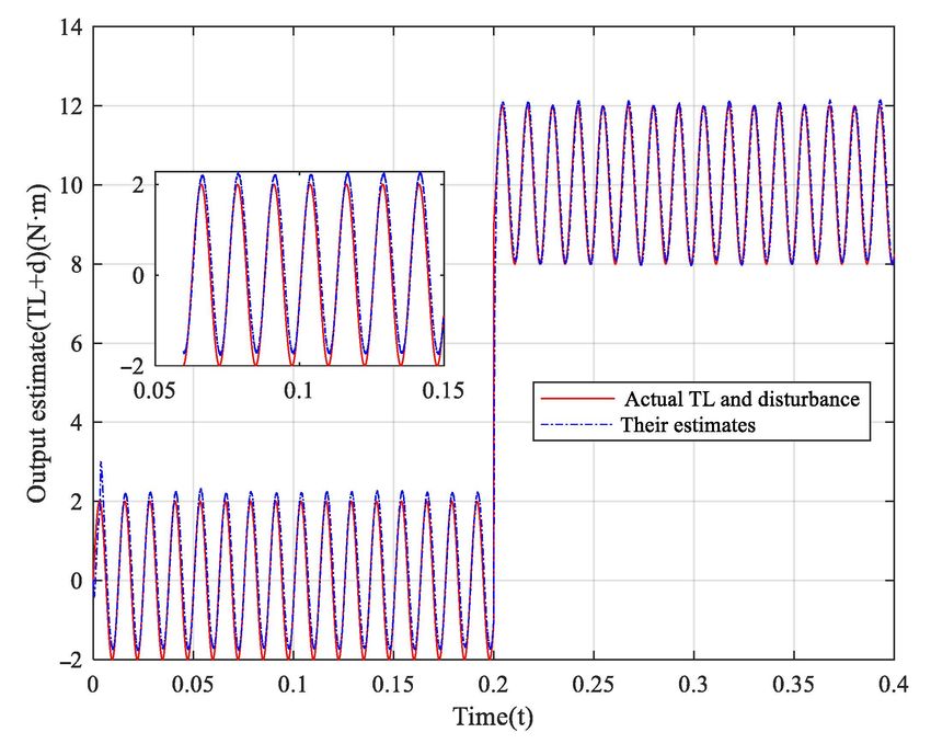
The speed response results with compensation and without compensation are shown in Figure 4,
respectively. One can obtain that the results with compensation are better than that without
compensation. The PD control is added to reduce overshoot. In addition, the estimates of load
and disturbance are utilized to reduce the impact of noise on the system.
Figure 4. The speed response results without compensation and with compensation in low speed
condition (the blue line indicating the speed response results with compensation, and the red line
indicating the speed response results without compensation).
From Figure 4, the Table 2 can be obtained. In the first column of the table, are the rising time,
setting time, overshoot of the speed curve, the lowest speed dropped when encountering torque
interference in 0.02 s, and the time to restore to the rated speed. The second and third columns of the
table are the values corresponding to the first column of the combined controller and the traditional
sliding mode controller designed in this paper. All the five indexes show that the control effect of the
proposed combined controller is very good.
Table 2. Simulation comparison performance (Nr = 300 r/s).
Items Combined Controller Traditional SMO
Rise time/ms 3.324 5.375
Setting time/ms 3.148 /
Overshoot/% 0.468 19.88
Lowest speed/rpm 290 193.7
Recovery time/ms 0.07 0.33
4.2. Simulation Results at High Speed
In this subsection, the parameters are set as same as the low speed condition. The ideal speed is
set as Nr = 1000r/s. While, the correction parameter θ = 1. Then the simulation results are shown in
Figures 5 and 6.
One can find out that the estimating result is worse than that under low-speed condition. It can
be concluded that the proposed method has better estimating performance under low-speed condition.
However, the speed-tracking performances are better than sliding mode control under both high-speed
condition and low-speed condition. In practical, the factors of load disturbance and measurement
noise can cause the change of system performance, even cause safety accident. Through the proposed
method, these problems can be reduced or avoided and maintain normal operation of the system.Appl. Sci. 2020, 10, 9006 11 of 13
Appl. Sci. 2020, 10, x FOR PEER REVIEW 11 of 13
Figure 5.
Figure The actual
5. The actual load
load and
and disturbance
disturbance with
with their
their estimates
estimates in
in high-speed
high-speed condition.
condition.
−
Figure 6. The speed response results without compensation and with compensation in high-speed
condition (the blue line indicating the speed response results with compensation, and the red line
indicating the speed response results without compensation).
The Table 3 can be obtained from Figure 6. It also shows that the control effect of the proposed
combined controller is very good. The decrease of overshoot is due to the addition of PD controller
based on sliding mode controller. The anti-torque capability is enhanced because the state observer is
Figure 6. The speed response results without compensation and with compensation in high-speed
used to estimate the torque disturbance, and then compensate it into the combined controller.
condition (the blue line indicating the speed response results with compensation, and the red line
indicating the speed response results without compensation).
Table 3. Simulation comparison performance (Nr = 1000 r/s).
The Table 3 can be obtained
Items from Figure 6. It also
Combined shows that Traditional
Controller the controlSMO
effect of the proposed
combined controller isRise
verytime/ms
good. The decrease of6.509
overshoot is due to the addition
7.609
of PD controller
based on sliding mode controller.
Setting time/msThe anti-torque 4.376
capability is enhanced because
/ the state observer
is used to estimate the Overshoot/%
torque disturbance, and then compensate it into the
0.498 combined controller.
38.184
Lowest speed/rpm 989.1 886.8
Recovery
Table 3.time/ms performance ( Nr 10000.28
Simulation comparison0.05 r / s ).
Items Combined Controller Traditional SMOAppl. Sci. 2020, 10, 9006 12 of 13
5. Conclusions
This paper investigates a combined controller base on sliding mode control method and PD control
strategy and a combined estimator based on slow time-varying estimation law and state observer.
The combined controller is used to improve the tracking performance and increase the response speed
of PMSM’s speed regulation by the analysis of PD control method. In addition, the estimator is
presented to reconstruct the disturbance and uncertainties caused by environment and simplified
model. Numerical examples based on Simulink model show the proposed algorithm can obtain a
superior dynamic performance with reducing the effect of load disturbances and overshoot. The
experimental implementation of the proposed algorithm, adopting optimization algorithm to select
parameters adaptively, researching the high-frequency low-voltage signal injection sensorless control
method, and modelling the PMSM system as a nonlinear model for research are planned to be carried
out in the future.
Author Contributions: Conceptualization, Y.T. and Y.C.; methodology, Y.C.; software, L.F.; validation, L.F.;
writing—original draft preparation, Y.T.; project administration, Y.T. and L.F.; funding acquisition, Y.C. All authors
have read and agreed to the published version of the manuscript.
Funding: This work is supported in part by the National Natural Science Foundation of China under Grant 61803055,
Grant 61633005, the Science and Technology Research Program of Chongqing Municipal Education Commission
under Grant No. KJQN201800720, Natural Science Foundation of Chongqing under Grant cstc2019jcyj-msxmX0222
and National Key R&D Program of China under Grant 2020YFB2009400.
Conflicts of Interest: The authors declare no conflict of interest.
References
1. Zhang, X.; Foo, G.H.B.; Rahman, M.F. A Robust Field-weakening Approach for Direct Torque and Flux
Controlled Reluctance Synchronous Motors with Extended Constant Power Speed Region. IEEE Trans. Ind.
Electron. 2019, 67, 1813–1823. [CrossRef]
2. Zhang, X.; Sun, L.; Zhao, K.; Sun, L. Nonlinear Speed Control for PMSM System Using Sliding-Mode Control
and Disturbance Compensation Techniques. IEEE Trans. Power Electron. 2013, 28, 1358–1365. [CrossRef]
3. Moon, H.T.; Kim, H.S.; Youn, M.J. A discrete-time predictive current control for PMSM. IEEE Trans. Power
Electron. 2003, 18, 464–472. [CrossRef]
4. Koiwa, K.; Kuribayashi, T.; Zanma, T.; Liu, K.Z.; Wakaiki, M. Optimal current control for PMSM considering
inverter output voltage limit: Model predictive control and pulse-width modulation. IET Electr. Power Appl.
2019, 13, 2044–2051. [CrossRef]
5. Kim, H.; Son, J.; Lee, J. A High-Speed Sliding-Mode Observer for the Sensorless Speed Control of a PMSM.
IEEE Trans. Ind. Electron. 2011, 58, 4069–4077.
6. Mohammad, M.; Ibne, R.M.B.; Farzana, R.L.; Rahman, T. High-Speed Current dq PI Controller for Vector
Controlled PMSM Drive. Sci. World J. 2014, 2014, 1–9.
7. Wang, X.; Xing, Y.; He, Z.; Yan, L. Research and Simulation of DTC Based on SVPWM of PMSM. Procedia Eng.
2012, 29, 1685–1689. [CrossRef]
8. Boukhezzar, B.; Siguerdidjane, H. Comparison between linear and nonlinear control strategies for variable
speed wind turbines. Control Eng. Pract. 2010, 18, 1357–1368. [CrossRef]
9. Quynh, N.V. The Fuzzy PI Controller for PMSM’s Speed to Track the Standard Model. Math. Probl. Eng.
2020, 2020, 1–20. [CrossRef]
10. Zhang, X.G.; Cheng, Y.; Zhao, Z.H.; He, Y.K. Robust Model Predictive Direct Speed Control for SPMSM Drives
Based on Full Parameter Disturbances and Load Observer. IEEE Trans. Power Electron. 2020, 35, 8361–8373.
[CrossRef]
11. Shanthi, R.; Kalyani, S.; Devie, P.M. Design and performance analysis of adaptive neuro-fuzzy controller for
speed control of permanent magnet synchronous motor drive. Soft Comput. 2020. [CrossRef]
12. Ge, Y.; Yang, L.H.; Ma, X.K. Adaptive sliding mode control based on a combined state/disturbance observer
for the disturbance rejection control of PMSM. Electr. Eng. 2020, 102, 1863–1879. [CrossRef]
13. Wang, Y.Q.; Feng, Y.T.; Zhang, X.G.; Liang, J. A New Reaching Law for Antidisturbance Sliding-Mode
Control of PMSM Speed Regulation System. IEEE Trans. Power Electron. 2020, 35, 4117–4126. [CrossRef]Appl. Sci. 2020, 10, 9006 13 of 13
14. Junejo, A.K.; Xu, W.; Mu, C.X.; Ismail, M.M.; Liu, Y. Adaptive Speed Control of PMSM Drive System Based A
New Sliding-Mode Reaching Law. IEEE Trans. Power Electron. 2020, 35, 12110–12121. [CrossRef]
15. Song, Z.; Mei, X.S.; Tao, T.T.; Xu, M.X. The Sliding-Mode Control Based on a Novel Reaching Technique for
Permanent Magnet Synchronous Motors. Electr. Power Compon. Syst. 2019, 47, 1–9. [CrossRef]
16. Cao, Y.H.; Wang, J.Z.; Shen, W. High-performance PMSM self-tuning speed control system with a low-order
adaptive instantaneous speed estimator using a low-cost incremental encoder. Asian J. Control 2020.
[CrossRef]
17. Morawiec, M.; Lewicki, A.; Wilczyński, F. Speed observer of induction machine based on backstepping and
sliding mode for low-speed operation. Asian J. Control 2020. [CrossRef]
18. Li, J.; Liao, Y. Model of Permanent Magnet Synchronous Motor Considering Saturation and Rotor Flux
Harmonics. Proc. CSEE 2011, 31, 60–66.
19. Sun, J.K.; Li, S.H. Disturbance observer based iterative learning control method for a class of systems subject
to mismatched disturbances. Trans. Inst. Meas. Control 2017, 39, 1749–1760. [CrossRef]
20. Zhang, K. Observer-Based Fault Estimation and Accommodation for Dynamic Systems. Ph.D. Thesis,
Nanjing University of Aeronautics and Astronautics, Nan Jing, China, 2012.
21. Yuan, L.; Hu, B.X.; Wei, K.Y.; Chen, S. Control Principle and MATLAB Simulation of Modern Permanent Magnet
Synchronous Motor; Beihang University Press: Beijing, China, 2016; pp. 70–71.
Publisher’s Note: MDPI stays neutral with regard to jurisdictional claims in published maps and institutional
affiliations.
© 2020 by the authors. Licensee MDPI, Basel, Switzerland. This article is an open access
article distributed under the terms and conditions of the Creative Commons Attribution
(CC BY) license (http://creativecommons.org/licenses/by/4.0/).You can also read