Design of SCMA Codebooks Using Differential Evolution - Unpaywall

Page created by Judy Hawkins
 
CONTINUE READING
Design of SCMA Codebooks Using Differential Evolution - Unpaywall
Design of SCMA Codebooks Using Differential Evolution
                                         Kuntal Deka1, Minerva Priyadarsini1 , Sanjeev Sharma2, and Baltasar Beferull-Lozano (Senior Member, IEEE)3
                                               1 Indian Institute of Technology Goa, India, 2 Indian Institute of Technology (BHU) Varanasi, India
                                          3 Department of Information and Communication Technology, University of Agder, Grimstad 4879, Norway

                                           Abstract—Non-orthogonal multiple access (NOMA) is a              multi-user detection is usually done by the message passing
                                        promising technology which meets the demands of massive             algorithm (MPA) [4].
                                        connectivity in future wireless networks. Sparse code multiple         Related work: The performance of an SCMA system is
                                        access (SCMA) is a popular code-domain NOMA technique. The
                                        effectiveness of SCMA comes from: (1) the multi-dimensional         mainly determined by the codebooks of the users. The opti-
                                        sparse codebooks offering high shaping gain and (2) sophisticated   mization of the codebooks for SCMA system is a convoluted
                                        multi-user detection based on message passing algorithm (MPA).      task as multiple users are interfering with multi-dimensional
                                        The codebooks of the users play the main role in determining the    complex vectors. In [3, 5], first, the optimum codebook for
                                        performance of SCMA system. This paper presents a framework         one user is designed. The remaining codebooks were obtained
                                        to design the codebooks by taking into account the entire system
arXiv:2003.03569v1 [cs.IT] 7 Mar 2020

                                        including the SCMA encoder and the MPA-based detector. The          by carrying out user-specific operations on the optimized
                                        symbol-error rate (SER) is considered as the design criterion       codebook. In [6] (referred to as “Zhang [6]”), the sum-rate
                                        which needs to be minimized. Differential evolution (DE) is used    was considered as one of the design criteria. First, a series of
                                        to carry out the minimization of the SER over the codebooks.        one-dimensional complex codewords were designed. Then the
                                        The simulation results are presented for various channel models.    angles of these codewords were changed with the objective
                                                                                                            of improving the sum-rate. The authors in [7] considered the
                                         Keywords SCMA, codebook design, differential evolution,            minimum Euclidean distance and the energy diversity of the
                                        message passing algorithm.                                          constellation points to obtain the optimum codebooks. Yu et
                                                                                                            al. (referred to as “Yu [8]”) designed SCMA codebooks based
                                                              I. I NTRODUCTION                              on the star quadrature amplitude modulation (QAM) constel-
                                                                                                            lations [8]. In [9], the authors designed codebooks for bit-
                                           The future wireless communication system will comprise           interleaved convolutionally-coded SCMA system. This design
                                        of enormous number of interconnected devices. The massive           was aided by the analysis based on EXtrinsic Information
                                        connectivity required in such situations cannot be fulfilled        Transfer (EXIT) chart. Sharma et al. [10] (referred to as
                                        by the multiple access schemes deployed so far. Earlier, 3G         “Sharma [10]”) designed the codebooks by maximizing the
                                        system used code division multiple access (CDMA), 4G used           mutual information and shaping gain. Kim et al. proposed a
                                        orthogonal frequency division multiple access (OFDMA) [1].          deep-learning-based method where, the codebook is dynami-
                                        All these technologies are based on orthogonal multiple access      cally designed with the objective of minimizing the bit error
                                        (OMA) principle. In OMA, the number of supported users is           rate (BER) [11].
                                        limited by the number of available orthogonal resources. The           Contributions: The existing codebook-design methods
                                        non-orthogonal multiple access (NOMA) technology provides           mainly focus on various geometric properties of the multi-
                                        a gateway for massive connectivity. It supports overloaded          dimensional constellations with little emphasis on detection.
                                        systems where the number of users is higher than the number         It is difficult to track the MPA-based detection process math-
                                        of orthogonal resources. NOMA techniques can be broadly             ematically. The factor graph is finite, not tree-like and it
                                        classified into two groups: power domain and code domain. In        contains short cycles. Due to these reasons, the techniques like
                                        power domain NOMA, different levels of powers are allocated         density evolution and EXIT chart cannot accurately character-
                                        to different users. In code domain NOMA, different code-            ize the MPA-based multi-user detection process. We propose
                                        words or signatures are used for different users. Low-density       to consider the symbol error rate (SER) as the cost function
                                        spreading (LDS) is a code-domain NOMA technique where,              which is to be minimized. The SER is one such quantity which
                                        a user’s symbol is multiplied with a distinct sparse spreading      takes into account every part of the multi-user system be it
                                        signature. This spread-ed sequence is mapped to modulation          Euclidean distance profile, product distance profile, MPA etc.
                                        constellation points for transmission [2]. Nikoupor et al. came     The reliability of the system is precisely reflected by the SER.
                                        up with the technique of sparse code multiple access (SCMA)         We adopt differential evolution (DE) for the minimization of
                                        in order to improve upon LDS [3]. In SCMA, the operations of        the SER as it is not a simple function of the codebooks.
                                        the spreading and the modulation mapping are merged. Based          DE is a flexible and effective evolutionary algorithm which is
                                        on a dedicated codebook, a symbol is directly mapped to a           used to solve complex optimization problems with real-valued
                                        sparse multi-dimensional codeword. Thus, SCMA provides              parameters [12, 13]. First, the structure of the codebooks is
                                        a better opportunity than LDS to attain high shaping gain.          represented with the help of a finite number of constellation
                                        Owing to the inherent sparsity in the code-domain NOMA, the         points. Then a DE-based optimization process is invoked to
Design of SCMA Codebooks Using Differential Evolution - Unpaywall
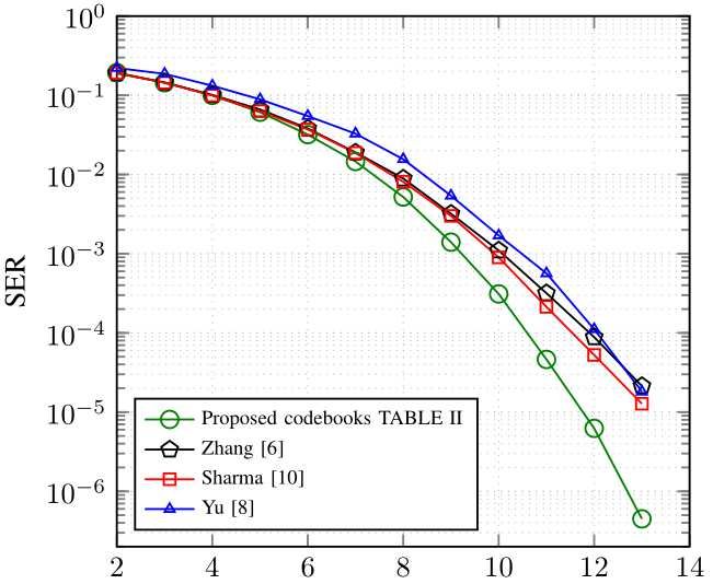
find the optimum constellation points. The codebooks for                minimum distance between any pair (xm , xn ) of codewords
the additive white Gaussian noise (AWGN) and Rayleigh                   in the entire SCMA system:
fading channels are designed. The SER performance of the
                                                                                                dE,min = min ||xm − xn ||.
proposed codebooks are compared with those of the existing                                                   m,n
ones. Moreover, various key parameters of the codebooks are             • Euclidean kissing number (τE ): It is defined as the number
computed and analyzed.                                                  of distinct codeword pairs with Euclidean distance equal to
   Outline: Section II describes the preliminaries such as              dE,min .
SCMA system model, important parameters of codebooks and                • Minimum product distance (dP,min ): The product distance
DE. The proposed method of codebook design is presented in              dm,n  between two codewords xm and xn is defined as
                                                                         P
Section III. The simulation results are presented and analyzed                                    Y
in Section IV. Section V concludes the paper.                                            dm,n
                                                                                          P   =        |xmj − xnj |
                                                                                                          j∈Jm,n
                       II. P RELIMINARIES
A. System Model                                                         where, Jm,n is the set of dimensions for which xmj 6= xnj .
                                                                        The minimum product distance dP,min is given by:
  A J × K SCMA system refers to an overloaded multi-
user scenario with J users and K resource elements. The                                             dP,min = min dm,n
                                                                                                                  P .
                                             J                                                                    m,n
overloading factor is given by λ = K           . A dedicated code-
book Cj containing M K-dimensional codewords: Cj =                      • Product Kissing Number (τP ): It is defined as the number of
{xj1 , xj2 , . . . , xjM } is assigned to every j th user. Each code-   distinct codeword pairs with product distance equal to dP,min .
word xjm is sparse with N non-zero complex components.                     The objective is to maximize dE,min , dP,min and minimize
Based on the assigned codebook Cj , log2 (M ) data bits                 τE , τP . In addition to these parameters, mutual information
are directly mapped to the K-dimensional codeword xj =                  between the received signal and the sum of the interfering
                  T                                         T
[xj1 , ..., xjK ] . The received signal y = [y1 , . . . yK ] is:        codewords is also a vital parameter. Suppose Y is the signal
                         J                                              received over one resource element. Let S represent the
                                                                        sum of the codewords of the df users interfering over that
                         X
                    y=         diag (hj ) xj + n                 (1)                                          df
                         j=1                                                             a total of M
                                                                        resource. We have                        distinct sum values for
                                                                        S as given by s1 , s2 , . . . , sM df . A high value of I(Y ; S)
                            T
where, hj = [h1 , . . . , hK ] is the channel gain vector for the       ensures successful recovery of the individual user’s data from
j th user and n is a complex K ×1 AWGN vector. The locations            the noisy sum value. Usually a lower bound IL on I(Y ; S) is
                                                                        considered1. IL for AWGN channel with noise variance N0 is
                                                                        given by [6]
                                                                                                                                                        
                                                                                                          1
                                                                                                                PM df PM df       
                                                                                                                                      1                2
                                                                         IL = log2 M df − log2 1 +
                                                                                                         M df     j=1   i=1    exp − 4N 0
                                                                                                                                          |s j − s i |     .
                                                                                                                        i6=j
                                                                                                                                                         (3)

                 Fig. 1: SCMA block diagram.
                                                                        B. Differential Evolution
of the non-zero elements of the codewords for the users can be
represented with the help of a factor matrix as shown in (2).             In DE, an initial set of SP random candidate solutions
The 1s present in the jth column specify the locations of the           or vectors {pi : i = 1, 2, . . . , SP } is generated. The length
non-zero components of the codewords for the jth user. The              of each vector is the same and it is denoted by D. New
matrix F can be alternatively represented by a factor graph as          generations are created iteratively using mutation, cross over
shown in Fig. 1. The degree of a resource node is denoted by            and selection process. During mutation, each vector pG  i , where
df . This specifies that df users interfere with each others over       G denotes the generation index, is selected as a primary parent.
one resource element. As the factor graph is sparse, MPA is             For each parent, a mutant vector is generated as follows:
used for multi-user detection.                                                                  uG
                                                                                               i = pr1 + α(pr2 − pr3 )                                 (4)
                          1 0 1 0 1 0
                         0 1 1 0 0 1                                  where, r1 , r2 , r3 are randomly selected distinct numbers dif-
                   F=   1 0 0 1 0 1
                                                             (2)       ferent from i and α is the scaling factor. uG  i is the secondary
                          0 1 0 1 1 0                                   parent generated from mutation. Cross-over is applied to
                                                                        primary and secondary parent to obtain the offspring vector
  The performance of an SCMA system is highly sensitive to              viG . Each component vik   G
                                                                                                     of viG = [vi1
                                                                                                                 G            G
                                                                                                                   , . . . , vik            G
                                                                                                                                 , . . . , viD ] is
the codebooks. In literature [14, 15], various key performance          inherited from either the primary or the secondary parent as
indicators (KPIs) have been considered for the design of multi-
dimensional constellations. A few of them are highlighted:
• Minimum Euclidean Distance (dE,min): It is defined as the               1 I(Y   ; S) or IL is related to the sum-rate [6].
Design of SCMA Codebooks Using Differential Evolution - Unpaywall
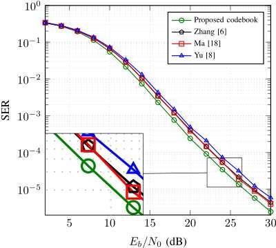
per the following rule:                                                  where, ai ∈ C, i = 1, . . . , 6.
                           (                                                In (6), 12 distinct complex numbers are created from 6 com-
                    G       uG
                             ik , if hk ≤ Cr                             plex numbers and their negative counterparts. It is preferable
                   vik   =   G
                            pik , otherwise                              to design the SCMA codebooks with the minimum possible
where, hk is a random number uniformly distributed over                  number of constellation points. This reduces the hardware
[0,1], Cr is the cross-over rate. The offspring is made to inherit       requirement in implementation.
                                                                            The one-dimensional codebooks can be assigned to all the
at least one component from the secondary parent to ensure
                                                                         resource nodes through a structure matrix satisfying Latin
that offspring is different from primary parent. The offspring
vector viG has to compete with the parent vector pG                      property [16]. This way of generating the entire set of the
                                                      k to get a
                                                                         codebooks was considered in [6, 17]. The structure matrix for
place in the next G + 1 generation. If vkG gives a lower cost
function than pG                                                         the 6 × 4 SCMA system is shown below:
                  k then the former replaces the later, else the                              o
                                                                                              C1 0 C2o 0 C3o 0
                                                                                                                            
primary parent vector exists in the next generation too, i.e.
                        (                                                                     0 C2o C3o 0          0 C1o 
                          viG , if f (viG ) ≤ f (pG
                                                  i )
                                                                                     FL =       o
                                                                                                                                    (7)
             pi
               (G+1)
                     =                                                                       C2 0        0 C1 0 C3o 
                                                                                                               o
                            G
                          pi , otherwise                                                              o
                                                                                                0 C1 0 C3 C2 0 o     o

where f (·) is the objective function that needs to be min-                The Latin property in (7) ensures that distinct one-
imized. The new generation performs at least as good as                  dimensional codebooks are assigned to the users overlapping
the best candidate of the previous generation. These steps               over any particular resource. Using FL , the set of all code-
are continued until some stopping criteria are satisfied. The            books can be generated as follows:
best vector from the current population is considered as the                              o                      o 
                                                                                           C1             0           C2,p
optimum vector.                                                                          0           C2o         C3o 
                                                                                   C1 = C2o  C2 =  0  C3 =  0 
                                                                                                                       
       III. P ROPOSED C ODEBOOK D ESIGN BASED              ON
                 D IFFERENTIAL E VOLUTION                                                   0            Co            0
                                                                                                      1o                     (8)
  Let C = {C1 , . . . , CJ } denote the set or the collection of                            0            C3            0
                                                                                         0            0          C1o 
the codebooks of all the users. The task of SCMA codebook                          C4 = C1o  C5 =  0  C6 = C3o 
                                                                                                                   
design is formulated as an optimization problem as follows:                                                o
                                                                                         C3o           C2,p          0
                                          Eb
               Copt = arg min f C;           ,F                          where, 0 is the all-zero row vector of length M = 4.
                                C        N0                  (5)
                                                                            In order to obtain more diversity and higher shaping gain,
                         s.t. ||c||2 = 1 ∀c ∈ C
                                                                         the authors in [6, 17] have proposed to carry out the di-
                                           Eb                            mensional permutation switching algorithm (DPSA). As per
where, f (·) is the SER at SNR N             0
                                               and F is the factor
graph matrix. Every K-dimensional codeword c present in                  DPSA, the permuted version of C2o denoted by C2,p  o
                                                                                                                               is used
                                                                                                                       o
the SCMA codebook system C is constrained to have unit                   in the codebooks C3 and C5 in place of C2 . We consider
                                                                           o
Euclidean norm.                                                          C2,p  = [−a4 , a3 , −a3 , a4 ]. With this dimensional permu-
   Note that an already-designed factor graph matrix F is fed            tation, using (6) in (8), the codebooks can be written as
to the optimization process in (5). Suppose the factor graph is          shown in TABLE I. Observe that the codebooks for the 6 × 4
regular with the resource node degree of df . Then, df users              TABLE I: Structure S of the codebooks C = {C1 , . . . , C6 }
overlap on a particular resource node. One needs to carefully                                                                
assign constellation points to these users. The task is to assign              
                                                                                 a1    a2    −a2     −a1         
                                                                                                                       0     0     0       0  
                                                                                   0  0  0  0                  a3  a4  −a4  −a3 
                                                                                                                                  
df distinct one-dimensional constellation2 codebooks to the
                                                                                                                                     
                                                                           C1 = a3  a4  −a4  −a3    C 2 =    0   0   0   0 
                                                                                                                   
df overlapping users. These codebooks may be represented
                                                                                                                                             
                                                                                   0     0     0       0               a1    a2    −a2     −a1
                                                                                                                                             
by C1o , C2o , . . . , Cdof , where the superscript ‘o’ signifies that
                                                                                                                              
                                                                               
                                                                                 −a4    a3    −a3     a4         
                                                                                                                        0     0     0       0  
these are one-dimensional. The size of the constellation is M .                   a5  a6  −a6  −a5  C4 =  0   0   0   0 
                                                                                                                               
                                                                          C3 =  0   0   0   0                a1  a2  −a2  −a1 
For example, consider the case of 6×4 SCMA system with                         
                                                                                                                  
                                                                                                                                                
                                                                                   0      0     0       0               a5    a6    −a6    −a5
                                                                                                                                              
the factor graph shown in Fig. 1 and the matrix in (2). Here,                                                                 
                                                                                  a5     a6    −a6    −a5               0     0     0       0 
df = 3 and M = 4. The three one-dimensional codebooks
                                                                               
                                                                                                                  
                                                                                                                                                
                                                                                   0   0   0   0  C6 = a1  a2  −a2  −a1 
                                                                                                                               
can be represented as follows:                                            C5 =  0   0   0   0                a5  a6  −a6  −a5 
                                                                               
                                                                                                                  
                                                                                                                                                
                                                                                  −a4    a3    −a3     a4                0     0     0       0
                                                                                                                                              
                    C1o = [a1 a2 − a2 − a1 ]
                    C2o = [a3 a4 − a4 − a3 ]                      (6)    SCMA system can be represented with the help of 6 complex
                    C3o   = [a5 a6 − a6 − a5 ]                           numbers ai , i = 1, . . . , 6. These complex numbers can be
                                                                         compactly represented by a = [a1 , . . . , a6 ]. Any particular
  2 One-dimensional codebook is assigned as only one resource node is    complex vector ai ,ai ∈ C6 refers to a particular set of
considered at a time.                                                    codebooks Ci = C1i , . . . , C6i . With these notations, the
Design of SCMA Codebooks Using Differential Evolution - Unpaywall
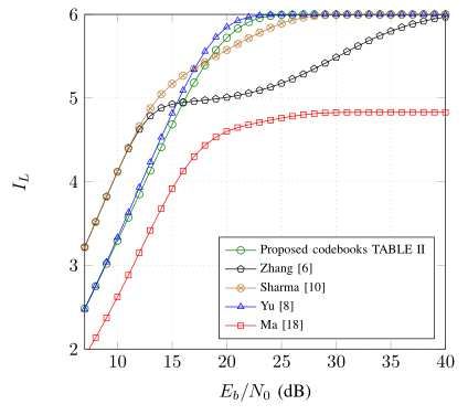
SCMA codebook design problem in (5) can now be written                   mum vector a which contains 6 complex numbers3. However,
as                                                                     DE is a real-valued optimization technique. Therefore, in this
                                     Eb                                  case, the number of real-valued variables to be optimized is
                aopt = arg min f a;                  (9)
                            a       N0                                   D = 12. The detailed steps for the DE-based codebook design
        
            Eb
                                                                        are presented in Algorithm 1. The inputs to the algorithm
where, f a; N     is the SER of the SCMA system defined
              0                                                          are the structure S for the codebooks as shown in TABLE I,
                 Eb
by a at SNR      N0. In the rest of the paper, for notational           SNR N  Eb
                                                                                     and the DE parameters: α, Cr ,SP and Imax .
                                                                                 0
                Eb                                                       The candidate vectors are stored in a population matrix P
brevity, f a; N  0
                      will be represented as f (a) with the
understanding that the SNR is fixed at a particular value during         in row-wise manner. The total number of candidate vectors
the optimization process. In (9), aopt is that vector a which            is SP . The size of P is SP × D. The elements of P
yields the optimum codebook Copt as per the structure given in           are initialized to random numbers uniformly distributed over
TABLE I. Moreover, we have the constraint that the Euclidean             [−1, 1]. Every row ps , s = 1, . . . , SP , of P corresponds to an
norm of every codeword is 1 although it is not explicitly                SCMA codebook system specified by the 6 complex numbers
mentioned in (9).                                                        as = [as,1 , . . . , as,6 ]. Suppose as,t = ars,t +acs,t i, t = 1, . . . , 6,
                                                                         where ars,t and acs,t are real uniform numbers in [−1, 1]. The
                                                                         sth row ps of P is given by
 Algorithm 1: Codebook design using differential evolution
                                                                                    ps = ars,1 , acs,1 , ars,2 , acs,2 , . . . , ars,6 , acs,6 .
                                                                                                                                             
                                                 Eb
  input : Codebook structure S (TABLE I),        N0
                                                    ,   DE parameters
          (α, Cr , SP and Imax )                                         The elements of P are normalized so that every codeword
  output: Codebooks Copt = {C1 , . . . , C6 }.
                                                                         in a codebook system has unit norm. Against each row
  Initialize the population matrix P to a matrix of size SP × D          ps , s = 1, . . . , SP , a trial vector u is generated with the
   having random numbers uniformly distributed over [−1, 1]
   where D = 12, Normalize these entries so that the every
                                                                         given values of the DE parameters: crossover rate (Cr ) and
   codeword of the codebook has unit norm;                               scaling factor (α). Algorithm 1 shows the detailed steps of the
  while termination criteria not fulfilled do                            generation of the trial vector u. The decision regarding the
       for i ← 1 to SP do                                                replacement of the current population vector ps by the trial
            Select three distinct vectors (rows) pr0 ,pr1 and pr2        vector u is made by computing the SER values for the two
              uniformly at random from P such that they are also
              different from pi ;                                        SCMA systems through Monte Carlo simulations. If the SER
            Generate an integer jrand uniformly at random from           value f (u) of the SCMA system defined by u is less than
              {1, 2, . . . , D};                                         the SER f (pi ) of the system defined by pi , then the current
            /* Generation of trial vector u                     */       population vector pi is set to u. In this way, every candidate
            for j ← 1 to D do                                            vector in P is examined and updated with the trial vectors
                 if rand[0,1] ≤ Cr or j = jrand then
                       uj,i = pj,r0 + α × (pj,r1 − pj,r2 )               if necessary. From the updated population P, the best vector
                         // Crossover and Mutation                       popt with the minimum SER value is identified. The above-
               else                                                      mentioned process is repeated unless f (popt ) is not changing
                      uj,i = pj,i                                        significantly during two consecutive iterations or the maximum
           Normalize the entries of u so that every codeword has         number of iterations are exhausted. The real numbers in popt
             unit norm.                                                  converted to the corresponding complex numbers to obtain
           /* Evaluation and Selection                          */       aopt . The complex numbers in aopt = [a1 , . . . , a6 ] are plugged
           Suppose Cu and Cpi are the two sets of the                    into S in TABLE I to obtain the optimum codebooks.
             codebooks for all users as per u and pi respectively.
           Run Monte Carlo simulation for the SCMA system                Example 1. Consider the case of J = 6, K = 4 SCMA system
                                                         Eb
             with the codebooks Cu and Cpi at SNR N       0
                                                            .            with constellation size M = 4. The structure given in TABLE I
             Suppose, f (u) and f (pi ) are the respective SER
                                                                         is used. The number of variables is D = 12. We can consider
             values ;
           if f (u) < f (pi ) then                                       SP = 20, Cr = 0.95 and α = 0.6. The population matrix P
                pi = u // Replace the ith row of P by u;                 may be initialized to the following 20 × 12 matrix:
      From the updated population matrix P, find the vector                                                                                     
                                                                              0.46 −0.53 −0.90 −0.22 −0.68  0.16 −0.34 −0.08 0.22 0.91 0.49 0.48
        (row) popt which yields the minimum value of SER;                   −0.02  0.90  0.44  0.08 −0.44  0.01  0.32 −0.84 0.10 0.24 0.82 0.12 
      If f (popt ) is not changing significantly from the previous
                                                                                                                                                
                                                                            −0.65 −0.62  0.80  0.11 −0.41 −0.15 −0.55  0.22 0.56 0.22 0.41 0.15 
                                                                         P=                                                                     .
                                                                                 ·     ·     ·     ·     ·     ·     ·     ·    ·    ·    ·    ·
        iteration or the maximum number of iterations Imax are
                                                                                                                                                
                                                                                                                                                
                                                                                ·     ·     ·     ·     ·     ·     ·     ·    ·    ·    ·    · 
        exhausted, then break from loop;                                         ·     ·     ·     ·     ·     ·     ·     ·    ·    ·    ·    ·

  Using pmin , form the optimum constellation vector                     Due to space constraint, only 3 rows out of 20 are shown. It
   aopt = [a1 , . . . , a6 ]. Then inserting a in S, the optimized set
   of the codebooks of all users Copt = {C1 , . . . , CJ } are
                                                                         may be verified that the norm of every codeword in P is 1.
   obtained. ;                                                              3 It is noteworthy that the proposed method of codebook design is universal
                                                                         in the sense that it can be applied to an SCMA system with any values of
                                                                         J and K. The structure as shown in TABLE I must be fed to the DE-based
  We solve (9) with the help DE. The job is to find the opti-            optimizer.
For every row of P, a trial vector is generated by carrying
out the mutation and the crossover operations as specified in
Algorithm 1. If the trial vector yields less SER than the current
row vector, then the current row is overwritten by the trial
vector. In this way every row of P is examined and updated if
needed. Suppose, finally, the population matrix P is as given
below where the first row is the best row pmin .
                                                                             
       −0.33 0.63 −0.83 0.43 0.71 0         −0.36 0     −0.42 −0.84 0.59 0.35
          ·    ·     ·    ·    · ·             · ·         ·     ·    ·    · 
P=                                                                           .
          ·    ·     ·    ·    · ·             · ·         ·     ·    ·    · 
           ·    ·     ·    ·    · ·             · ·         ·     ·    ·    ·

Then the solution of (9) is given by the following:
aopt = [−0.33 + 0.63i, −0.83 + 0.43i, 0.71, −0.36, −0.42 − 0.84i, 0.59 + 0.35i] .

Using the above aopt in TABLE I, we can generate the code-
books for the SCMA system. TABLE II shows these codebooks
in Section IV.
Remark 1. Although the proposed scheme appears to be SNR-
dependent, the codebooks optimized at a high SNR are found
to work well at different SNR values. In practice, we fix an
SNR where the SER is around 10−3 . The results for different                                             Fig. 2: aopt for AWGN channel.
SNR values are not shown here due to space constraint.
                                                                                        TABLE II: Codebooks optimized for AWGN channel
   Complexity Analysis: Observe from Algorithm 1 that during                             
                                                                                         
                                                                                                                                                    
                                                                                            −0.3318 + 0.6262i −0.8304 + 0.4252i 0.8304 − 0.4252i 0.3318 − 0.6262i 
                                                                                                                                                                           

each cycle of DE, the objective functions (SERs) for the
                                                                                                                                                                           
                                                                                                     0                     0                   0                  0
                                                                                                                                                                   
                                                                                     C1 =                                                                           
                                                                                                 0.7055             −0.3601            0.3601           −0.7055     
current population and the trial vector are computed. The SER
                                                                                         
                                                                                                                                                                           
                                                                                                     0                     0                   0                  0
                                                                                                                                                                           
                                                                                                                                                                         
computation is a time-consuming process       due to fact that the
                                                                                                                                                    
                                                                                         
                                                                                                    0                     0                   0                  0         
                                                                                                                                                                            
                                                                                                  0.7055               −0.3601              0.3601             −0.7055
                                                                                                                                                                          
complexity of the MPA is O M df . Thus, the complexity
                                                                                                                                                  
                                                                                     C2 =                                                                          
                                                                                         
                                                                                                    0                   0                 0                0        
                                                                                                                                                                            
                                                                                            −0.3318 + 0.6262i −0.8304 + 0.4252i 0.8304 − 0.4252i 0.3318 − 0.6262i
                                                                                                                                                                           
of proposed algorithm is higher than some of the existing                                                                                                          
                                                                                                  0.3601               0.7055             −0.7055              −0.3601
codebook designing methods. However, note that the codebook
                                                                                         
                                                                                                                                                                           
                                                                                                                                                                            
                                                                                            −0.4202 − 0.8350i 0.5933 + 0.3548i −0.5933 − 0.3548i 0.4202 + 0.8350i
                                                                                                                                                                    
                                                                                     C3 = 
                                                                                                     0                    0                   0                   0
design is a one-time and offline task. It does not add to the real-                                                                                                
                                                                                                                                                                           
                                                                                                     0                    0                   0                   0
                                                                                                                                                                           

time complexity of the system. Therefore, the proposed DE-
                                                                                                                                                                    
                                                                                         
                                                                                                   0                     0                    0                   0          
                                                                                                                                                                              
                                                                                                    0                     0                    0                   0
                                                                                                                                                                    
based codebook design method is feasible in practical scenario.                     C4 = 
                                                                                         
                                                                                         
                                                                                                                                                     
                                                                                          −0.3318 + 0.6262i −0.8304 + 0.4252i  0.8304 − 0.4252i  0.3318 − 0.6262i
                                                                                                                                                                            
                                                                                                                                                                              
                                                                                            −0.4202 − 0.8350i     0.5933 + 0.3548i     −0.5933 − 0.3548i 0.4202 + 0.8350i
                                                                                                                                                                             

                     IV. S IMULATION R ESULTS
                                                                                                                                                                   
                                                                                         
                                                                                           −0.4202  − 0.8350i    0.5933 +  0.3548i  −0.5933  −  0.3548i   0.4202 + 0.8350i 
                                                                                                                                                                            
                                                                                                     0                    0                   0                   0
                                                                                                                                                                   
                                                                                     C5 =                                                                           
  The simulations are carried out to evaluate the performance                            
                                                                                         
                                                                                         
                                                                                                    0
                                                                                                  0.3601
                                                                                                                        0
                                                                                                                       0.7055
                                                                                                                                            0
                                                                                                                                          −0.7055
                                                                                                                                                                0
                                                                                                                                                               −0.3601
                                                                                                                                                                           
                                                                                                                                                                            
                                                                                                                                                                            
of the proposed codebooks. For comparison, the following                                 
                                                                                         
                                                                                                   0
                                                                                                             
                                                                                                                          0
                                                                                                                                    
                                                                                                                                               0
                                                                                                                                                         
                                                                                                                                                                   0
                                                                                                                                                                            
                                                                                                                                                                              
                                                                                                                                                                              
codebooks are considered: • “Zhang [6]” • “Sharma [10]”                                                       −0.8304 + 0.4252i  0.8304 − 0.4252i  0.3318 − 0.6262i
                                                                                            −0.3318 + 0.6262i
                                                                                                                                                                     
                                                                                    C6 = −0.4202 − 0.8350i  0.5933 + 0.3548i  −0.5933 − 0.3548i 0.4202 + 0.8350i
                                                                                         
• “Yu [8]” • “Ma [18]” (Chapter 12 of [18]). As per the
                                                                                                                                                                             
                                                                                                    0                     0                    0                   0
                                                                                                                                                                             

thumb rules provided in [19, 20], the DE parameters are set to:
SP = 20, D = 12, Cr = 0.95, α = 0.6 and Imax = 80. The
simulations are done for uncoded transmission over AWGN                             in Fig. 3. The SER plots for the other codebooks are also
and flat Rayleigh fading channels.                                                  presented. Observe that the proposed codebooks outperform
                                                                                    the others by a significant margin. Specifically, there is cod-
A. AWGN channel                                                                     ing gain of about 1.4 dB at SER=10−5 over the next best
  First the results for the AWGN channel are presented.                             codebooks (“Sharma [10]”). The performance of “Ma [18]”
An SCMA system with J = 6, K = 4 and M = 4 is                                       over AWGN channel is not satisfactory. Therefore, its SER
                                           Eb
considered. Algorithm 1 is run at N         0
                                               = 10 dB to find the                  plot is not shown in Fig. 3. However, “Ma [18]” yields good
optimum vector aopt . The complex numbers of aopt and their                         results over Rayleigh fading channel which is presented later
negative versions are shown in Fig. 2. With this value of                           in this section.
aopt = [a1 , a2 , a3 , a4 , a5 , a6 ], the optimum codebooks are                       The SER performance of the various codebooks can be
generated using the structure S shown in TABLE I. These                             studied and justified by carrying out the mutual information
codebooks are shown in TABLE II. Observe that Euclidean                             analysis as mentioned in Section II-A. We plot the lower
norm of every codeword is 1.                                                        bound IL on mutual information for various codebooks in
  The SER performance of the proposed codebooks are eval-                           Fig. 4. Observe that in the SNR region below 16 dB, “Shamra
uated through Monte Carlo simulations and these are shown                           [10]” and “Zhang [6]” provide higher values of IL than the
B. Fading channel
                                                                     In this case, each user observes independent Rayleigh fading
                                                                  channel coefficients over the resource elements. The same
                                                                  SCMA framework with J = 6, K = 4, M = 4 and the
                                                                  structure S given in TABLE I is considered. Algorithm 1 is
                                                                                Eb
                                                                  executed at N   0
                                                                                    = 17 dB. It yields the optimum constellation
                                                                  vector aopt which are plotted in Fig. 5. The complex numbers

Fig. 3: SER performance of the SCMA system using various
codebooks for J = 6 and K = 4 in AWGN channel.

                                                                                        Fig. 5: aopt for fading channel.

                                                                  in aopt = [a1 , . . . , a6 ] are put in S. The resulting codebooks are
                                                                  shown in TABLE III. Observe that the optimized codebooks
                                                                  for the fading channel are different from those for the AWGN
                                                                  channel. This signifies that the codebook design problem
                                                                  depends on the underlying channel model.

                                                                       TABLE III: Codebooks optimized for fading channel
                                                                                                                                                     
                                                                       
                                                                         −0.3344 − 0.7316i −0.5754 + 0.2224i         0.5754 − 0.2224i     0.3344 + 0.7316i  
                                                                                  0                      0                    0                    0
                                                                                                                                                     
                                                                  C1 =                                                             
                                                                          0.4153 − 0.4248i   0.4680 + 0.6328i  −0.4680 − 0.6328i −0.4153 + 0.4248i
                                                                                                                                                             
                                                                       
                                                                                                                                                             
                                                                                  0                      0                    0                    0
                                                                                                                                                             
                                                                                                                                                     
                                                                                 0                      0                    0                    0          
Fig. 4: Lower bound on the mutual information for various
                                                                                                                                                             
                                                                         0.4153 − 0.4248i   0.4680 + 0.6328i  −0.4680 − 0.6328i −0.4153 + 0.4248i
                                                                  C2 =                                                                                
                                                                                  0                      0                    0                    0
codebooks.
                                                                       
                                                                       
                                                                                                                                                       
                                                                                                                                                              
                                                                          −0.3344 − 0.7316i −0.5754 + 0.2224i         0.5754 − 0.2224i     0.3344 + 0.7316i
                                                                                                                                                             
                                                                                                                                                   
                                                                        
                                                                           −0.4680 − 0.6328i 0.4153 − 0.4248i −0.4153 + 0.4248i 0.4680 + 0.6328i           
                                                                            −0.1492 − 0.5839i 0.7759 − 0.1713i −0.7759 + 0.1713i 0.1492 + 0.5839i
                                                                                                                                                    
                                                                    C3 = 
proposed codebooks. However, the IL for “Yu [8]” and the                
                                                                        
                                                                                   0                   0                 0                 0        
                                                                                                                                                             
                                                                                    0                     0                   0                   0
                                                                                                                                                            
proposed codebooks reach the maximum value of 6 quicker                 
                                                                                  0
                                                                                             
                                                                                                          0
                                                                                                                    
                                                                                                                               0
                                                                                                                                         
                                                                                                                                                   0
                                                                                                                                                            
                                                                                                                                                             
than the other codebooks. Observe that IL for “Yu [8]” is
                                                                                                                                                            
                                                                                   0                      0                    0                   0
                                                                                                                                                    
                                                                   C4 =                                                             
                                                                          −0.3344 − 0.7316i −0.5754 + 0.2224i  0.5754 − 0.2224i  0.3344 + 0.7316i
                                                                                                                                                            
slightly higher than that for the proposed codebooks in the
                                                                        
                                                                                                                                                            
                                                                           −0.1492 − 0.5839i      0.7759 − 0.1713i    −0.7759 + 0.1713i 0.1492 + 0.5839i
                                                                                                                                                            
                                                                                                                                                   
range of 15-20 dB. They reach the maximum value almost                  
                                                                        
                                                                        
                                                                            −0.1492 −
                                                                                    0
                                                                                       0.5839i
                                                                                              
                                                                                                  0.7759 −
                                                                                                          0
                                                                                                            0.1713i
                                                                                                                   
                                                                                                                      −0.7759 +
                                                                                                                              0
                                                                                                                                 0.1713i
                                                                                                                                        
                                                                                                                                          0.1492 +
                                                                                                                                                  0
                                                                                                                                                    0.5839i
                                                                                                                                                           
                                                                                                                                                             
                                                                                                                                                             
                                                                    C5 = 
at the same SNR of 24 dB. However, as described later in                
                                                                        
                                                                                   0
                                                                                              
                                                                                                        0
                                                                                                                   
                                                                                                                            0
                                                                                                                                        
                                                                                                                                                0
                                                                                                                                                           
                                                                                                                                                           
                                                                                                                                                             
                                                                            −0.4680 − 0.6328i 0.4153 − 0.4248i −0.4153 + 0.4248i 0.4680 + 0.6328i
                                                                                                                                                            
this section, the Euclidean distance and the product distance           
                                                                                  0
                                                                                             
                                                                                                          0
                                                                                                                    
                                                                                                                               0
                                                                                                                                         
                                                                                                                                                   0
                                                                                                                                                            
                                                                                                                                                             
profiles of “Yu [8]” are poorer than those of the proposed one.
                                                                                                                                                            
                                                                           −0.3344 − 0.7316i −0.5754 + 0.2224i  0.5754 − 0.2224i  0.3344 + 0.7316i
                                                                                                                                                     
                                                                   C6 =  −0.1492 − 0.5839i  0.7759 − 0.1713i  −0.7759 + 0.1713i 0.1492 + 0.5839i
This observation reinforces the superior performance of the             
                                                                        
                                                                        
                                                                                   0                      0                    0                   0
                                                                                                                                                             
                                                                                                                                                             

proposed DE-based codebooks. Also note that the IL for “Ma
[18]” cannot climb up to the maximum value. This justifies          The SER performance of the proposed codebooks along
the poor performance of “Ma [18]” over the AWGN channel.          with those of the other existing ones are shown in Fig. 6.
The progress of Algorithm 1 with increasing iteration is
                                                                 depicted in Fig. 7. The minimum SER corresponding to the
                                                                 best vector/row in the population matrix P as updated in
                                                                 the current iteration is plotted against the iteration number.
                                                                 Observe from Fig. 7 that the minimum SER tends to settle
                                                                 down at a value after 20 iterations. We have observed similar
                                                                 progression of the DE-based algorithm in the case of AWGN
                                                                 channel. However, due to space constraint, the plot for AWGN
                                                                 channel is not included in the paper.
                                                                    The values of the KPIs mentioned in Section II-A are shown
                                                                 in TABLE IV for various codebooks. “Zhang [6]” has the best
                                                                 Euclidean distance profile. Its dE,min is the highest and τE
                                                                 is the lowest. Proposed codebook (AWGN) has the highest
                                                                 dP,min , however the τP is not the lowest. The Euclidean
                                                                 distance parameters for “Ma [18]” are the worst since dE,min
                                                                 is the lowest and τE is the highest. Its poor performance over
                                                                 AWGN channel can be attributed to this fact. However, its
                                                                 product distance profile is impressive. Its dP,min is not the
                                                                 lowest and τP has the lowest value. However, it is difficult
                                                                 to justify the reported SER performances completely with the
Fig. 6: SER performance of the SCMA system using various
                                                                 help of the KPIs mentioned in TABLE IV.
codebooks for J = 6 and K = 4 in Rayleigh fading channel.
                                                                             TABLE IV: Key performance indicators
                                                                            Proposed   Proposed
                                                                                                  Zhang [6]   Sharma [10]   Yu [8]   Ma [18]
Observe that the proposed codebooks produce the best results.               (AWGN)     (Fading)
At SER=10−5 , we experience a coding gain of about 1.5 dB          dE,min   0.8966     0.8625      1.0171       0.9976      0.5351   0.3883
over the next best methods: “Zhang [6]” and “Ma [18]”. We            τE        4          4           2            2           2        4
                                                                   dP,min   0.1103     0.0595      0.0810       0.0544      0.0379   0.0448
also evaluate the SER performance of the proposed codebooks          τP        4          4           4            4           2        2
designed for the AWGN channel. However, the performance
is not satisfactory and inferior to “Zhang [6]”, “Ma [18]” and
                                                                   These KPIs only partially characterize the SCMA system.
“Yu [8]”. This observation reiterates the well known fact that
                                                                 The SCMA system is a complicated mult-user scenario where
the optimum constellation for AWGN may not be optimum
                                                                 the detection is carried out by the sophisticated MPA. These
for Rayleigh fading channel and vice versa [14].
                                                                 KPIs fail to take the MPA-based detection process into ac-
                                                                 count. Thus they are inadequate to facilitate a conclusive
                                                                 comparative analysis of various codebooks.
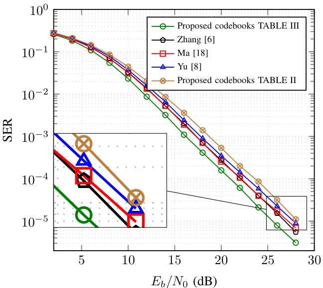
                                                                   The above codebooks can be enlarged to build J = 8, K =
                                                                 4 SCMA systems with 200% overloading factor. We consider
                                                                 the following factor matrix:
                                                                                                               
                                                                                     1 0 1 0 1 0 1 0
                                                                                    0 1 1 0 0 1 1 0
                                                                              F=  1 0 0 1 0 1 0 1.
                                                                                                                

                                                                                     0 1 0 1 1 0 0 1
                                                                    The 3rd and the 4th columns are repeated as the 8th and
                                                                 7th ones respectively. The constellation points for C3 and C4
                                                                 are exchanged between the 7th and the 8th users. The SER
                                                                 performances of these codebooks are shown in Fig. 8 for
                                                                 Rayleigh fading channel. In this case also, the proposed DE-
                                                                 based codebooks yield the best result.

                                                                                         V. C ONCLUSIONS
                                                                    This paper presented a method to design the codebooks for
                                                                 an SCMA system. The constellation points are designed with
Fig. 7: Minimum SER versus iteration in Rayleigh fading          the objective of minimizing the SER. The SER is considered
           Eb
channel at N 0
               = 17 dB during differential evolution process.    as it directly reflects the effectiveness of the system to detect a
tions design,” IEEE Transactions on Communications, vol. 66, no. 11,
                                                                                         pp. 5292–5304, Nov 2018.
                                                                                  [10]   S. Sharma, K. Deka, V. Bhatia, and A. Gupta, “SCMA codebook based
                                                                                         on optimization of mutual information and shaping gain,” in 2018 IEEE
                                                                                         Globecom Workshops (GC Wkshps), Dec 2018, pp. 1–6.
                                                                                  [11]   M. Kim, N. Kim, W. Lee, and D. Cho, “Deep Learning-Aided SCMA,”
                                                                                         IEEE Communications Letters, vol. 22, no. 4, pp. 720–723, April 2018.
                                                                                  [12]   R. Storn and K. Price, “Differential Evolution – A Simple and Efficient
                                                                                         Heuristic for global Optimization over Continuous Spaces,” Journal of
                                                                                         Global Optimization, vol. 11, no. 4, pp. 341–359, Dec 1997. [Online].
                                                                                         Available: https://doi.org/10.1023/A:1008202821328
                                                                                  [13]   S. Das and P. N. Suganthan, “Differential evolution: A survey of
                                                                                         the state-of-the-art,” IEEE Transactions on Evolutionary Computation,
                                                                                         vol. 15, no. 1, pp. 4–31, Feb 2011.
                                                                                  [14]   J. Boutros and E. Viterbo, “Signal space diversity: a power- and
                                                                                         bandwidth-efficient diversity technique for the rayleigh fading channel,”
                                                                                         IEEE Transactions on Information Theory, vol. 44, no. 4, pp. 1453–
                                                                                         1467, July 1998.
                                                                                  [15]   M. Vameghestahbanati, I. D. Marsland, R. H. Gohary, and
                                                                                         H. Yanikomeroglu, “Multidimensional constellations for uplink SCMA
                                                                                         systemsa comparative study,” IEEE Communications Surveys Tutorials,
                                                                                         vol. 21, no. 3, pp. 2169–2194, thirdquarter 2019.
                                                                                  [16]   J. Denes and A. D. Keedwell, Latin squares: New developments in the
                                                                                         theory and applications. Elsevier, 1991.
                                                                                  [17]   K. Xiao, B. Xia, Z. Chen, B. Xiao, D. Chen, and S. Ma, “On capacity-
Fig. 8: SER performance of the SCMA system using various                                 based codebook design and advanced decoding for sparse code multi-
codebooks for J = 8 and K = 4 in Rayleigh fading channel.                                ple access systems,” IEEE Transactions on Wireless Communications,
                                                                                         vol. 17, no. 6, pp. 3834–3849, June 2018.
                                                                                  [18]   Mojtaba Vaezi, Zhiguo Ding and H. Vincent Poor , Ed., Multiple
                                                                                         Access Techniques for 5G Wireless Networks and Beyond. Springer
user’s data in interference-limited environment. First the struc-                        International, 2019.
ture of the codebooks is fixed using a finite number of complex                   [19]   K. Price, R. Storm, and J. Lampinen, Differential Evolution. Springer-
                                                                                         Verlag Berlin Heidelberg, 2005.
numbers. The minimization of the SER over these variables                         [20]   Anyong Qing, Differential Evolution: Fundamentals and Applications
is accomplished with the help of DE. The optimum complex                                 in Electrical Engineering. Wiley IEEE, 2009.
numbers are then used to form the desired codebooks. It is
found that the codebook-design task is a channel-dependent
affairs. The SER performance of the proposed codebooks for
the AWGN and the fading channels are compared with those
of other existing codebooks in literature. This comparison
established the superiority of the proposed method over others.
                              R EFERENCES
 [1] L. Dai, B. Wang, Y. Yuan, S. Han, I. Chih-Lin, and Z. Wang, “Non-
     orthogonal multiple access for 5G: solutions, challenges, opportunities,
     and future research trends,” IEEE Communications Magazine, vol. 53,
     no. 9, pp. 74–81, 2015.
 [2] R. Hoshyar, F. P. Wathan, and R. Tafazolli, “Novel low-density signature
     for synchronous CDMA systems over AWGN channel,” IEEE Transac-
     tions on Signal Processing, vol. 56, no. 4, pp. 1616–1626, April 2008.
 [3] H. Nikopour and H. Baligh, “Sparse code multiple access,” in 2013
     IEEE 24th Annual International Symposium on Personal, Indoor, and
     Mobile Radio Communications (PIMRC), Sept 2013, pp. 332–336.
 [4] F. R. Kschischang, B. J. Frey, and H. . Loeliger, “Factor graphs and
     the sum-product algorithm,” IEEE Transactions on Information Theory,
     vol. 47, no. 2, pp. 498–519, Feb 2001.
 [5] M. Taherzadeh, H. Nikopour, A. Bayesteh, and H. Baligh, “SCMA
     codebook design,” in 2014 IEEE 80th Vehicular Technology Conference
     (VTC2014-Fall), Sep. 2014, pp. 1–5.
 [6] S. Zhang, K. Xiao, B. Xiao, Z. Chen, B. Xia, D. Chen, and S. Ma,
     “A capacity-based codebook design method for sparse code multiple
     access systems,” in 2016 8th International Conference on Wireless
     Communications Signal Processing (WCSP), Oct 2016, pp. 1–5.
 [7] M. Alam and Q. Zhang, “Designing optimum mother constellation and
     codebooks for SCMA,” in IEEE International Conference on Commu-
     nications (ICC). IEEE, 2017, pp. 1–6.
 [8] L. Yu, X. Lei, P. Fan, and D. Chen, “An optimized design of SCMA
     codebook based on star-QAM signaling constellations,” in 2015 In-
     ternational Conference on Wireless Communications Signal Processing
     (WCSP), Oct 2015, pp. 1–5.
 [9] J. Bao, Z. Ma, M. Xiao, T. A. Tsiftsis, and Z. Zhu, “Bit-interleaved coded
     SCMA with iterative multiuser detection: Multidimensional constella-
You can also read