Prey-Predator Model with a Nonlocal Bistable Dynamics of Prey - MDPI
←
→
Page content transcription
If your browser does not render page correctly, please read the page content below
mathematics
Article
Prey-Predator Model with a Nonlocal Bistable
Dynamics of Prey
Malay Banerjee 1, *,† , Nayana Mukherjee 1,† and Vitaly Volpert 2,†
 1   Department of Mathematics and Statistics, IIT Kanpur, Kanpur 208016, India
 2   Institut Camille Jordan, UMR 5208 CNRS, University Lyon 1, 69622 Villeurbanne, France;
     volpert@math.univ-lyon1.fr
 *   Correspondence: malayb@iitk.ac.in; Tel.: +91-0512-259-6157
 †   These authors contributed equally to this work.

 Received: 5 February 2018; Accepted: 5 March 2018; Published: 8 March 2018

 Abstract: Spatiotemporal pattern formation in integro-differential equation models of interacting
 populations is an active area of research, which has emerged through the introduction of nonlocal
 intra- and inter-specific interactions. Stationary patterns are reported for nonlocal interactions in prey
 and predator populations for models with prey-dependent functional response, specialist predator
 and linear intrinsic death rate for predator species. The primary goal of our present work is to
 consider nonlocal consumption of resources in a spatiotemporal prey-predator model with bistable
 reaction kinetics for prey growth in the absence of predators. We derive the conditions of the Turing
 and of the spatial Hopf bifurcation around the coexisting homogeneous steady-state and verify the
 analytical results through extensive numerical simulations. Bifurcations of spatial patterns are also
 explored numerically.

 Keywords: prey-predator; nonlocal consumption; Turing bifurcation; spatial Hopf bifurcation;
 spatio-temporal pattern

1. Introduction
     Investigation of spatiotemporal pattern formation leads to understanding of the interesting
and complex dynamics of prey-predator populations. Reaction-diffusion systems of equations are
conventionally used to study such dynamics. Various forms of reaction kinetics in the spatiotemporal
model give rise to a wide variety of Turing patterns as well as non-Turing patterns including
traveling wave [1–5] and spatiotemporal chaos [6,7]. Such patterns can be justified ecologically
with the help of the field data and experiments which confirm the presence of patches in the
prey-predator distributions. For example, Gause [8] has shown the importance of spatial heterogeneity
for the stabilization and long term survival of species in the laboratory experiment on growth of
paramecium and didinium. Luckinbill [9,10] has also studied the effect of dispersal on stability as well
as persistence/extinction of population over a longer period of time. Based on these data, works are
done where the prey-predator models with spatial distribution are considered for various ecological
processes [11], such as plankton patchiness [12–14], semiarid vegetation patterns [15], invasion by
exotic species [16,17] etc. (see also [18–21]). Such models have been successful in proving long
term coexistence of both prey and predator populations along with formation of stationary or time
dependent localized patches with periodic, quasi-periodic and chaotic dynamics [6,7].
     The classical representation of two species interacting populations including the spatial aspect,
consists of a reaction-diffusion system of equations in the form of two nonlinear coupled partial
differential equations,

Mathematics 2018, 6, 41; doi:10.3390/math6030041                          www.mdpi.com/journal/mathematics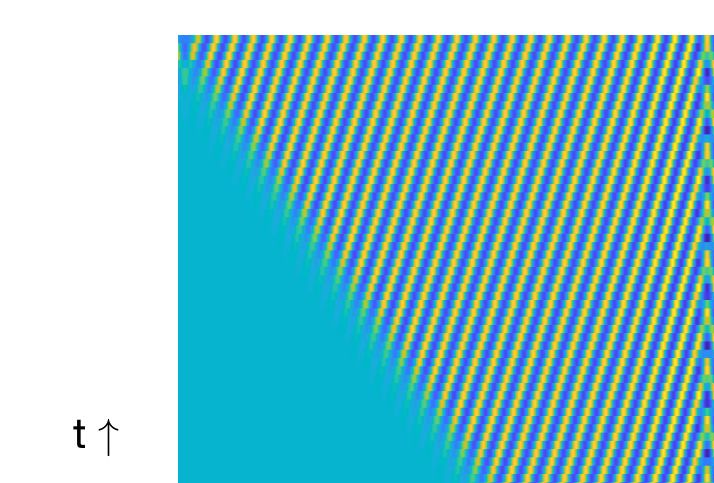
Mathematics 2018, 6, 41                                                                               2 of 13

                                        ∂u           ∂2 u
                                               = du       + F1 (u, v),                                   (1)
                                        ∂t           ∂x2
                                        ∂v           ∂2 v
                                               =   dv 2 + F2 (u, v)                                      (2)
                                        ∂t           ∂x
with non-negative initial conditions and appropriate boundary conditions. Population densities of prey
and predator species at the spatial location x and time t are denoted by u( x, t) and v( x, t), respectively.
The nonlinear functions F1 and F2 represent the interactions among individuals of the two species.
The diffusion coefficients du and dv represent the rate of random movement of individuals of the two
species within the considered domain.
     A wide variety of spatiotemporal patterns are described by these models, namely, traveling
wave, periodic traveling wave, modulated traveling wave, wave of invasion, spatiotemporal chaos,
stationary patchy patterns etc. [20–23]. Among all these, only stationary patchy pattern results in
due to Turing instability, represents a stationary in time but non-homogeneous in space distribution.
A stable co-existence of both species occurs due to formation of localized patches where the average
population of each species remains unaltered in time. Whereas the other patterns are time dependent
with the individuals of both species following continuously changing resources.
     The general assumption for consumption of resources in the spatiotemporal models of interacting
populations is taken to be local in space. In other words, it is supposed that the individuals
consume resources in some areas surrounding their average location. Whereas nonlocal consumption
of resources is more general since it incorporates the interspecific competition for food [24–26].
Such modifications enables the explanation of emergence and evolution of biological species as
well as speciation in a more appropriate manner [27–31]. The models with nonlocal consumption
of resources present complex dynamics for the single species models [28,29,32–35] as well as for
competition models including two or more species [32,36–38]. Furthermore, such complex dynamics
cannot be found in the corresponding local models.
     Interesting results are obtained due to the introduction of nonlocal consumption of prey by
predator in a reaction-diffusion system with Rosenzweig-McArthur type reaction kinetics [39].
Contrary to the local model where Turing patterns are not observed, this model satisfies the Turing
instability conditions and gives rise to Turing patterns under proper assumptions on parameters. Other
than this, existence of non-Turing patterns like traveling wave, modulated traveling wave, oscillatory
pattern and spatiotemporal chaos are also observed for the nonlocal model. Some of the non-Turing
patterns are reported for the nonlocal model with the modified Lotka-Volterra reaction kinetics [39,40].
     In order to introduce the prey-predator model with a nonlocal bistable dynamics of prey, let us
recall the classical models for the single population. Single species population model with the logistic
growth law is described by the following ordinary differential equation, assuming homogeneous
distribution of the species over their habitat,

                                             du
                                                = ru(k − u),                                             (3)
                                             dt
where r and k denote the intrinsic growth rate and carrying capacity, respectively. Introducing
multiplicative Allee effect in this single population growth model, the above equation becomes

                                       du
                                          = ru(k − u)(u − l ),                                           (4)
                                       dt
where l is the Allee effect threshold satisfying the restriction 0 < l < k [41–45]. This equation
accounts for two significant feedback effects: positive feedback due to cooperation at low population
density and negative feedback arising through the competition for limited resources at high population
density [46]. In the framework of this formulation, the cooperation and competition mechanisms are
described by the linear factors (u − l ) and (k − u), respectively. Introduction of the Allee effect through
a multiplicative term has a significant drawback since it represents a product of cooperation at the
Mathematics 2018, 6, 41                                                                                3 of 13

low population density and competition at the high population density. In this case, cooperation and
competition influence each other, and their effects cannot be considered independently (see [46,47]
for detailed discussion). The per capita growth rate is described by the factor r (k − u)(u − l ) which is
positive for l < u < k, it is an increasing function for l < u < k+    l
                                                                      2 , and a decreasing function for
k+l
 2 < u < k. To overcome such situations, an additive form of the per capita growth rate function,
proposed by Petrovskii et al. [47], is given by

                                      du
                                         = u ( f (u) − σ − g(u)) ,                                        (5)
                                      dt

where the functions f (u) and g(u) describe population growth due to the reproduction and density
dependent enhanced mortality rate, respectively. Here σ is the natural mortality rate independent of
population density. Depending upon appropriate parametrization and assumption for the functional
forms, the above model describes various types of single species population growth. In particular, if
we choose f (u) = µu and g(u) = ηu2 then we get the growth Equation (4) from (5) with appropriate
relations between two sets of parameters (r, k, l ) and (µ, σ, η ). With a different type of parametrization,
f (u) = abu and g(u) = au2 we can obtain the single species population growth model with sexual
reproduction [34,35,48] as follows

                                         du
                                            = au2 (b − u) − σu,                                           (6)
                                         dt
where a is the intrinsic growth rate, b is the environmental carrying capacity and σ is the density
independent natural death rate. Introducing the nonlocal consumption of resources and random
motion of the population, we get the following integro-differential equation model,
                                                         Z ∞
                            ∂2 u( x, t)

              ∂u( x, t)                     2
                        = d             + au ( x, t) b −     φ( x − y)u(y, t)dt − σu( x, t),              (7)
                ∂t             ∂x2                        −∞

where φ(z) is an even function with a bounded support and d is the diffusion coefficient. The kernel
                                                 R∞
function is normalized to satisfy the condition −∞ φ(z)dz = 1. It shows the efficacy of consumption of
resources as a function of distance (x − y). The integral describes the total consumption of resources at the
point x by the individuals located at y ∈ (−∞, ∞). This model shows bistability since the corresponding
temporal model has two stable steady-states 0 and u+ separated by an unstable steady-state u− [34].
     Based on this model, we are interested to study pattern formation described by the nonlocal
reaction-diffusion system of prey-predator interaction with the bistable reaction kinetics of prey in
the absence of predators which are specialist in nature following Holling type-II functional response.
We will obtain the conditions of the Turing instability and of the spatial Hopf bifurcation in Section 2.
Section 3 describes spatiotemporal pattern formation observed in numerical simulations. Here we
also present bifurcation diagrams for the model with nonlocal consumption. Main outcomes of this
investigation are summarized in the discussion section.

2. Stability Analysis
    In this section, we will introduce the prey-predator models without and with nonlocal
consumption term and will study stability of the positive homogeneous stationary solution.

2.1. Local Model
      We consider the following reaction-diffusion system for the prey-predator interaction:

                               ∂u          ∂2 u                        αuv
                                     = d1       + au2 (b − u) − σ1 u −     ,                              (8)
                               ∂t          ∂x2                         κ+u
                               ∂v          ∂2 v    βuv
                                     =   d2 2 +          − σ2 v,                                          (9)
                               ∂t          ∂x     κ+u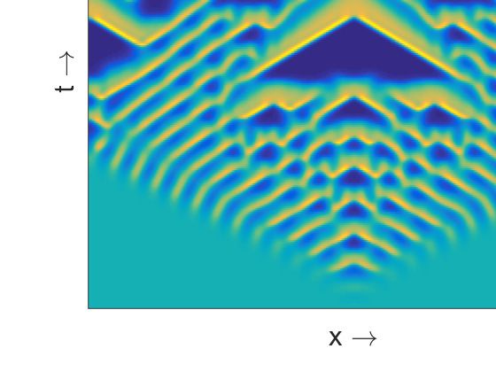
Mathematics 2018, 6, 41                                                                                      4 of 13

subjected to a non-negative initial condition and the periodic boundary condition. The consumption
of prey by the predator follows the Holling type-II functional response, α is the rate of consumption
of prey by an individual predator, κ is the half-saturation constant and β is the rate of conversion
of prey to predator biomass. Furthermore, β/α is the conversion efficiency with the value between
0 and 1, consequently β < α. The reproduction of prey is proportional to the second power of the
population density specific for sexual reproduction. In the absence of predator (α = 0) dynamics of
prey is described by a bistable reaction-diffusion equation.
     The coexistence (positive) equilibrium E∗ (u∗ , v∗ ) of the corresponding temporal model

                               du                               αuv
                                     = au2 (b − u) − σ1 u −         ≡ f (u, v),                               (10)
                               dt                               κ+u
                               dv         βuv
                                     =        − σ2 v ≡ g(u, v),                                               (11)
                               dt         κ+u

is given by the equalities

                                     κσ2          κ + u∗
                           u∗ =            , v∗ =        ( au∗ (b − u∗ ) − σ1 ) ,                             (12)
                                    β − σ2          α

and associated feasibility conditions

                                                      aκσ2                κσ2
                                0 < σ2 < β, 0 < σ1 <                  b−
                                                     β − σ2              β − σ2
which provide the positiveness of solutions.
    Here we briefly present the local asymptotic stability condition of E∗ for the temporal
model (10)–(11) that will be required afterwards. Linearizing the nonlinear system (10)–(11) around E∗
we can find the associated eigenvalue equation

                                            λ2 − a11 λ − a12 a21 = 0,

where

         a11 = f u (u∗ , v∗ ), a12 = f v (u∗ , v∗ ) < 0, a21 = gu (u∗ , v∗ ) > 0, a22 = gv (u∗ , v∗ ) = 0.

     Two eigenvalues of the above characteristic equation have negative real parts if a11 < 0 and
hence E∗ is locally asymptotically stable for a11 < 0. The stationary point E∗ loses its stability through
the super-critical Hopf bifurcation if a11 = 0.
     It is well known that the models of the form (8)–(9), that is for which a22 = 0, are unable to
produce any Turing pattern as the Turing instability conditions cannot be satisfied [40]. However these
type of models are capable to produce non-Turing pattern if the temporal parameter values are well
inside the Hopf-bifurcation domain [6]. The spatiotemporal prey-predator models with a specialist
predator and linear death rate for predator population can produce spatiotemporal chaos, wave of
chaos, modulated traveling wave, wave of invasion and their combinations if the spatial domain is
large enough [7].

2.2. Nonlocal Model
   Under the assumption that prey can move from one location to another one to access the resources,
model (8)–(9) can be extended to the model with nonlocal consumption of resources:

                              ∂u           ∂2 u                            αuv
                                     = d1       + au2 (b − J (u)) − σ1 u −     ,                              (13)
                              ∂t           ∂x2                             κ+u
                              ∂v           ∂2 v    βuv
                                     =   d2 2 +          − σ2 v,                                              (14)
                              ∂t           ∂x     κ+u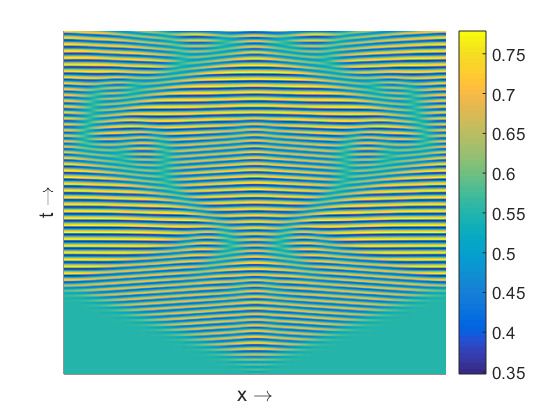
Mathematics 2018, 6, 41                                                                                     5 of 13

subjected to a non-negative initial condition and the periodic boundary condition. Here
                           Z ∞
                                                             (
                                                                  1
                   J (u) =      φ( x − y)u(y, t)dy,   φ(y) =     2M , | y | ≤ M .
                            −∞                                    0 , |y| > M

     Various forms of kernel functions are considered in literature. Here we consider the step
function for simplicity of mathematical calculations [49]. This step function means that the nonlocal
consumption is confined within the range 2M, and the efficacy of consumption inside this range
is constant.
     We will analyze stability of the homogeneous steady-state (u∗ , v∗ ). We consider the perturbation
around it in the form

                      u( x, t) = u∗ + e1 eλt+ikx ,   v( x, t) = v∗ + e2 eλt+ikx ,       |e1 |, |e2 |  1.
      The characteristic equation writes as | H − λI | = 0 where
                                         "                                          #
                                                           kM
                                             a1 − au2∗ sinkM  − d1 k 2    − a2
                                  H =                                                                        (15)
                                                        b1               − d2 k 2

and
                                               αu∗ v∗              αu∗           βu∗ v∗
                     a1 = abu∗ − au2∗ +                 2
                                                          , a2 =        , b1 =             .                 (16)
                                             (κ + u ∗ )          κ + u∗        (κ + u ∗ )2

      Therefore, the characteristic equation becomes as follows:

                                        λ2 − Γ(k, M )λ + ∆(k, M) = 0,                                        (17)

where
                                                 sin kM
                              Γ(k, M)= a1 − au2∗         − ( d1 + d2 ) k 2 ,                                 (18)
                                                  kM
                                           2 sin kM
                             ∆(k, M) =   au∗          − a1 + d1 k d2 k2 + a2 b1 .
                                                                 2
                                                                                                             (19)
                                               kM

    The homogeneous steady-state is stable under space dependent perturbations if the following
two conditions are satisfied:

                                         Γ(k, M) < 0, ∆(k, M ) > 0                                           (20)

for all positive real k and M. The homogeneous steady-state loses its stability through the spatial
Hopf bifurcation if Γ(k H , M ) = 0, ∆(k H , M) > 0 for some k H , and through the Turing bifurcation if
Γ(k T , M ) < 0, ∆(k T , M ) = 0 for some k T .

2.3. Spatial Hopf Bifurcation
     First, we find the spatial Hopf bifurcation threshold in terms of the parameter d2 . It is important to
note that Γ(k, M ) < 0 and ∆(k, M ) > 0 as M → 0+ if we assume that (u∗ , v∗ ) is locally asymptotically
stable for the temporal model (10)–(11). One can easily verify that lim M→0+ Γ(k, M ) = a11 and
lim M→0+ ∆(k, M ) = − a12 a21 . For some suitable M if one can find a unique value k ≡ k H such
that Γ(k, M) = 0 then k H is the critical wavenumber for the spatial Hopf bifurcation. This critical
wavenumber can be obtained by solving the following two equations simultaneously:

                                                          ∂
                                        Γ(k, M ) = 0,        Γ(k, M) = 0.                                    (21)
                                                          ∂k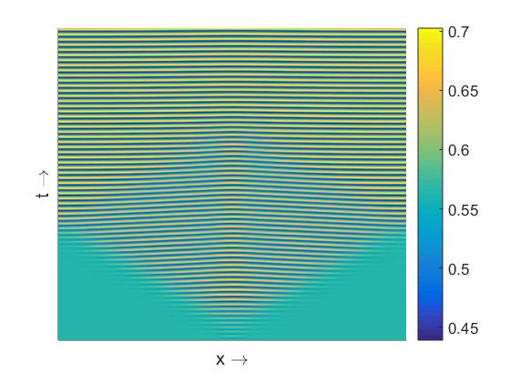
Mathematics 2018, 6, 41                                                                                  6 of 13

      Using the expression of Γ(k, M), we find d2 from the equation Γ(k, M ) = 0:

                                                  1             2 sin kM         2
                                     d2 ( k ) =        a 1 − au ∗        − d 1 k     .                    (22)
                                                  k2                kM

      Substituting this expression into the second equation in (21) we get:

                                                                     sin kM
                                     2a1 + au2∗ cos kM − 3au2∗              = 0.                          (23)
                                                                       kM
      Equation (23) can have more than one positive real root depending upon the values of parameters.
It is necessary to verify that the corresponding values of d2 (k) are positive. We choose the root k H for
which d2 (k H ) is the minimal positive number, and ∆(k H , M ) > 0.
      Consider, as example, the following values of parameters:

           a = 1, b = 1, σ1 = 0.1, α = 0.335, κ = 0.4, β = 0.335, σ2 = 0.2, d1 = 1.                       (24)

     Then u∗ = 0.593, v∗ = 0.419, and Equation (23) possesses only one positive root k = 0.297 for
M = 6. From (22), we find d2 = 0.51. Since ∆(0.51, 6) = 0.0094, these values of k and d2 correspond
to the desired spatial Hopf bifurcation thresholds, k H = 0.297, d2H = 0.51.
     Furthermore, Γ(k, 6) > 0 for d2 < d2H . Hence the spatial Hopf bifurcation takes place as d2
crosses the critical threshold d2H from higher to lower values. Therefore, oscillatory in space and
time patterns emerging due to the spatial Hopf bifurcation are observed below the stability boundary.
The spatial Hopf bifurcation curve in the ( M, d2 )-parameter space is shown in Figure 1. Spatiotemporal
patterns for parameter values lying in the spatial Hopf domain is presented in Figure 3a.

                          1.6

                          1.4

                          1.2
                                                      Turing domain
                           1
                     d2

                          0.8     Stable                                     Turing spatial Hopf
                                  homogeneous                                domain
                          0.6     steady-state

                          0.4
                                              Spatial Hopf domain

                          0.2
                            5.5                   6               6.5                    7         7.5
                                                                 M

                  Figure 1. Turing and Hopf stability boundaries in the (M, d2 )-parameter plane.

2.4. Turing Pattern for Nonlocal Prey-Predator Model
     Next, we discuss the Turing bifurcation condition and we assume that lim M→0+ Γ(k, M) < 0 and
lim M→0+ ∆(k, M ) > 0. These conditions provide stability of the homogeneous steady-state under
space independent perturbations. The critical wavenumber and the corresponding Turing bifurcation
threshold in terms of d2 can be obtained as a solution of the following two equations:

                                                             ∂
                                         ∆(k, M ) = 0,          ∆(k, M) = 0.                              (25)
                                                             ∂k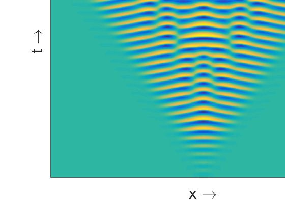
Mathematics 2018, 6, 41                                                                                                           7 of 13

          From ∆(k, M ) = 0, we get

                                                                              a2 b1
                                        d2 ( k ) =               h                              i.                                 (26)
                                                                                           kM
                                                           k2        a1 − d1 k2 − au2∗ sinkM

          Substituting this expression into the second equation in (25), we obtain

                                         2                                         sin kM
                                     4d1 k − 2a1 +          au2∗          cos kM +               = 0.                              (27)
                                                                                     kM

       This equation can have more than one positive root. From now on, we assume that all parameter
values are fixed except for M and d2 . Suppose that for a chosen value of M, (27) admits a finite number
of positive roots, k1 , k2 , · · · , k m . The corresponding values of d2 (k i ) in (26) are not necessarily positive.
The Turing bifurcation threshold d2T is given by the minimal positive value d2 (k i ), and k T is the value
of k i for which the minimum is reached.
       Let us consider the same set of parameters as in the previous subsection except for d1 = 0.4.
An interesting feature of the Turing bifurcation curve is that it is not smooth when plotted in the
( M, d2 )-parameter plane (Figure 2). The point of non-differentiability arises around M = 12.65. For
M = 12.5, we find four positive roots of (27), k1 = 0.038, k2 = 0.470, k3 = 0.638 and k4 = 0.786.
The corresponding values d2 (k jr ) are positive for the last three roots, d2 (k2 ) = 0.198, d2 (k3 ) = 0.235
and d2 (k4 ) = 0.199. Hence we find the Turing bifurcation threshold d2T = 0.198, corresponding
to k2 (Figure 2b). Next, if we choose M = 12.7, then we find k1 = 0.0378, k2 = 0.465, k3 = 0.620,
k4 = 0.781, and d2 (k2 ) = 0.201, d2 (k3 ) = 0.232, d2 (k4 ) = 0.189 are positive d2 -values. Hence, the
Turing bifurcation threshold d2T = 0.189 corresponds to k4 (Figure 2c). Hence, the point where the
stability boundary is not smooth correspond to the sudden change of the location of the feasible root
of Equation (27).

         0.3                                              1.5                                                   1.5

                                                            1                                                     1
        0.25
                                               ∆(k,M) →

                                                                                                     ∆(k,M) →

                                                          0.5                                                   0.5
 d2 →

         0.2
                                                            0                                                     0
        0.15                                              -0.5                                                  -0.5

         0.1                                               -1                                                    -1

                                                                                                                            k→
               5     10         15      20                       0              0.5              1                     0    0.5         1
                          M→                                                    k→
                          (a)                                                  (b)                                         (c)

          Figure 2. Turing bifurcation curve on the (M, d2 )-parameter plane (a). Stationary Turing patterns exist
          above the bifurcation curve. The functions ∆(k, 12.5) (b) and ∆(k, 12.7) (c).The root corresponding to
          the Turing instability is shown in green.

     Finally, it is important to mention that the choice of parameters (24) leads to an interesting
scenario for which the spatial Hopf and Turing bifurcation curves intersect. The two curves are shown
in Figure 1 for d1 = 1, and they divide the parametric domain into four different regions. Spatial
patterns produced by the prey population for parameter values taken from spatial Hopf domain and
Turing domain are presented in Figure 3a,b. In order to emphasize the fact that the stationary Turing
pattern can be obtained for equal diffusion coefficients, we set d1 = d2 = 1 and observe a periodic in
space and stationary in time solution (see Figure 3b). Various spatio-temporal patterns are observed
for the values of parameters at the intersection of Turing and Hopf instability regions. Some of them
are described in Section 3.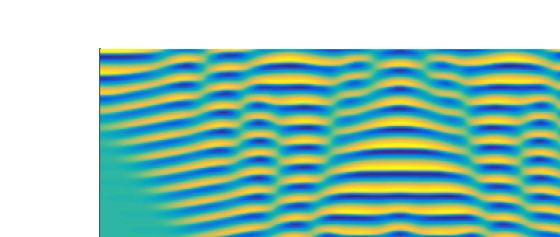
Mathematics 2018, 6, 41 8 of 13
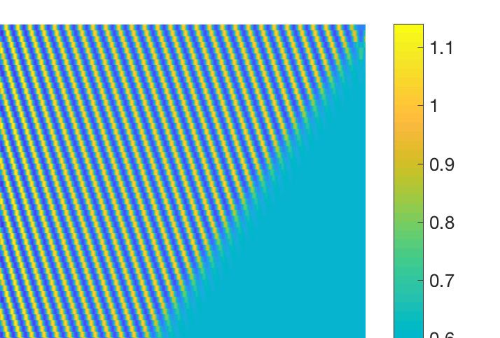
(a) (b)
Figure 3. (a) Resulting spatio-temporal patterns produced by the nonlocal model (13)–(14) for d2 = 0.3,
M = 6.5 and other parameter values as mentioned in the text. (b) Stationary pattern produced by the
prey population for d1 = 1, d2 = 1 and M = 6, other parameters are mentioned at text.
3. Spatiotemporal Patterns
In this section, we study nonlinear dynamics of the prey-predator model without and with
nonlocal term in the equation for prey population. We present the results of numerical simulations
performed with a finite difference approximation of systems (8)–(9) and (13)–(14).
3.1. Patterns Produced by the Model (8)–(9)
In this subsection, we consider the non-Turing patterns described by system (8)–(9) in the interval
− L ≤ x ≤ L with non-negative initial condition and periodic boundary condition. Results presented
here are obtained for L = 200. We consider a small perturbation around the homogeneous steady-state
at the center of the domain as initial condition. The values of parameters are as follows
a = 1, b = 1, σ1 = 0.1, α = 0.4, κ = 0.4, σ2 = 0.2, d1 = 1, d2 = 1, (1)
and the value of β will vary.
It is known [6,7,16,26,50] that the prey-predator models with specialist predator can manifest time
dependent spatial patterns if the parameters of the reaction kinetics are far inside the temporal Hopf
domain. In this case, the temporal Hopf-bifurcation threshold is β ∗ = 0.339, that is E∗ is stable for
β < β ∗ , and it is unstable otherwise.
Solutions homogeneous in space and oscillatory in time are observed for β > β ∗ but close to it.
The spatiotemporal pattern presented in Figure 4a is almost homogeneous in space but oscillatory in
time for the value of β close to the temporal Hopf bifurcation threshold. For larger values of β we find
spatiotemporal patterns periodic both in space and time (Figure 4b) and symmetric around x = 0.
This symmetry is maintained due to the choice of symmetric initial condition. With the increase of β
we observe various complex aperiodic spatiotemporal regimes (Figure 4c). They are characterized by
specific triangular patterns resulting from the merging of two peaks in the population density moving
towards each other.
This model is capable to produce other type of spatiotemporal patterns, such as the traveling
wave, periodic travelling wave, wave of invasion, wave of chaos similar to the prey-predator model
with Rosenzweig-MacArthur reaction kinetics [26] but those results are beyond the scope of this work
and will be addressed in the future.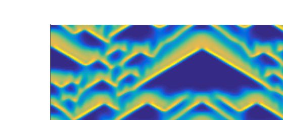
Mathematics 2018, 6, 41                                                                                 9 of 13

                              (a)                                              (b)

                              (c)                                              (d)

                              (e)                                              (f)

      Figure 4. Spatiotemporal patterns (prey density) produced by the model (8)–(9) are presented in the
      left column for the parameter values as mentioned at the text and (a) β = 0.342; (c) β = 0.3445;
      (e) β = 0.36. Corresponding distribution of prey and predator population over space at t = 1000 are
      presented in the right column, see (b), (d), (f).

3.2. Effect of Nonlocal Consumption
     We will now analyze how the nonlocal term influences dynamics of the prey-predator model.
Nonlinear dynamics of prey-predator system with nonlocal consumption of resources by prey is
summarized in the diagram in Figure 5a. Parameter regions with different regimes are shown on the
( M, β)-plane for the values of other parameters given in (1). For small β, predator disappears while
the population of prey is either homogeneous in space or it forms a spatially periodic distribution. For
large β, both population go to extinction. More interesting behavior is observed for the intermediate
values of β. This can be homogeneous or inhomogeneous in space, stationary or non-stationary in time
solutions. Some of the spatiotemporal patterns are shown in Figure 6. For M sufficiently small these
patterns become similar to those presented in Figure 4. For M large enough, both prey and predator
densities represent stationary periodic in space distributions (similar to Figure 3b). Figure 5b shows a
similar diagram in the case of different diffusion coefficients of prey and predator, d1 = 0.7, d2 = 0.5,
with the same values of other parameters. The region of spatiotemporal patterns exists here for a
narrower interval of β while the regions of stationary patterns and of extinction change their shape.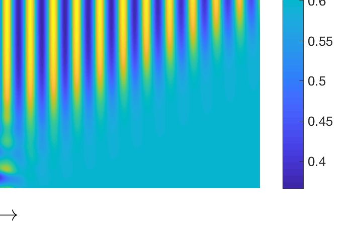
Mathematics 2018, 6, 41                                                                                   10 of 13

                              (a)                                                           (b)

      Figure 5. Bifurcation diagram in ( M, β)-parameter space for fixed parameters a = 1, b = 1, σ1 = 0.1,
      α = 0.4, κ = 0.4 and σ2 = 0.2. (a) d1 = 1, d2 = 1; (b) d1 = 0.7, d2 = 0.5.

                   (a)                                                     (b)                    (c)

      Figure 6. Spatio-temporal patterns produced by the nonlocal model with parameter values as
      mentioned at (1) with β = 0.342 and (a) M = 0; (b) M = 4; (c) M = 6.

Multiplicity of Stationary Solutions
     Another interesting aspect of the stationary patterns arising through the Turing bifurcation for the
spatiotemporal model with nonlocal interaction term is the existence of multiple stationary solutions
for a particular value of M. We have used forward and backward numerical continuation method
to determine the range of M for the stationary patterns with different periodicity (Figure 7). Fixed
parameter values are same as (1) except d1 = 0.4 and d2 = 0.2. For example, stationary pattern
with 33 patches (over a spatial domain of size L = 200) exists for 2 ≤ M ≤ 4.5, with 32 patches for
2.5 ≤ M ≤ 5, and so on.

                                                             35
                              Number of stationary patches

                                                             30

                                                             25

                                                             20

                                                             15

                                                             10

                                                             5
                                                                  5   10         15   20   25
                                                                           M

      Figure 7. Stationary patterns with various number of patches exist for a range of nonlocal consumption
      (M) is plotted. Parameter values are same as in (24) except d1 = 0.4 and d2 = 0.2.
Mathematics 2018, 6, 41 11 of 13
4. Discussion
In this work we study a prey-predator model with a bistable nonlocal dynamics of prey. Without
the interaction with predator, the prey density is described by a bistable reaction-diffusion equation
taking into account the Allee effect or the sexual reproduction of population. In this case, the
reproduction rate is proportional to the second power of the population density. The dynamics
of the prey population changes due to introduction of nonlocal consumption of resources. The
main difference compared to the results of conventional local consumption is that the positive stable
equilibrium may become unstable resulting in the appearance of stationary in time but periodic in
space solutions.
The interaction with predator provides an additional factor that influences the dynamics of
solutions. If we characterize this interaction by the parameter β, which determines the reproduction
rate in the equation of predator density, then we can identify three main types of behavior depending
on its value (Figure 5). If it is sufficiently small then the predator population vanishes since the
reproduction is not enough to overcome the mortality. If this parameter is too large, then both
populations go to extinction, particularly due to the bistability of the prey dynamics. Both populations
coexist in a relatively narrow interval of the interconnection parameter. There are three different types
of patterns inside this parameter domain. The homogeneous in space equilibrium can be stable or
it can lose its stability resulting in the emergence of spatiotemporal patterns. They are observed for
limited values of the parameter M which determines the range of nonlocal consumption. If the range
of nonlocal consumption is sufficiently large, then both populations represent a periodic in space
distribution. Such solutions are specific for nonlocal consumption with a large range, in particular for
the single prey population. Thus, nonlocal consumption takes over spatiotemporal oscillations specific
for the local prey-predator dynamics. Let us note that there is multiplicity of stationary patterns for
the same values of parameters. This effect is specific for the problems with nonlocal interaction [39].
Spatiotemporal oscillations are specific for the prey-predator dynamics [6,7,16,26,40,50]. Here we
observe the dynamics with “triangular” patterns (Figure 4) appearing when two pulses move towards
each other and merge. Nonlocal consumption of resources modifies these patterns.
Some questions related to the prey-predator dynamics with nonlocal bistable model for prey
remain beyond the scope of this work. We have not discussed here travelling waves and pulses that
can also be observed in such models. We will study them in the subsequent work.
Author Contributions: M.B. and V.V. proposed the formulation of the problem; N.M. performed the numerical
simulations; M.B. and N.M. analyzed the results; all authors participated in the preparation of the manuscript.
Conflicts of Interest: The authors declare no conflict of interest.
References
1. Dunbar, S.R. Travelling wave solutions of diffusive Lotka-Volterra equations. J. Math. Biol. 1983, 17, 11–32.
2. Dunbar, S.R. Travelling waves in diffusive predator-prey equations: Periodic orbits and point-to-periodic
heteroclinic orbits. SIAM J. Appl. Math. 1986, 46, 1057–1078.
3. Sherratt, J.A. Periodic travelling waves in cyclic predator-prey systems. Ecol. Lett. 2001, 4, 30–37.
4. Sherratt, J.A.; Smith, M. Periodic travelling waves in cyclic populations: Field studies and reaction diffusion
models. J. R. Soc. Interface 2008, 5, 483–505.
5. Volpert, V.; Petrovskii, S.V. Reaction-diffusion waves in biology. Phys. Life Rev. 2009, 6, 267–310.
6. Petrovskii, S.V.; Malchow, H. A minimal model of pattern formation in a prey-predator system. Math. Comp.
Model. 1999, 29, 49–63.
7. Petrovskii, S.V.; Malchow, H. Wave of chaos: New mechanism of pattern formation in spatio-temporal
population dynamics. Theor. Pop. Biol. 2001, 59, 157–174.
8. Gause, G.F. The Struggle for Existence; Williams and Wilkins: Baltimore, MD, USA, 1935.
9. Luckinbill, L.L. Coexistence in laboratory populations of Paramecium aurelia and its predator Didinium nasutum.
Ecology 1973, 54, 1320–1327.Mathematics 2018, 6, 41 12 of 13
10. Luckinbill, L.L. The effects of space and enrichment on a predator-prey system. Ecology 1974, 55, 1142–1147.
11. Fasani, S.; Rinaldi, S. Factors promoting or inhibiting Turing instability in spatially extended prey-predator
systems. Ecol. Model. 2011, 222, 3449–3452.
12. Huisman, J.; Weissing, F.J. Biodiversity of plankton by oscillations and chaos. Nature 1999, 402, 407–410.
13. Levin, S.A.; Segel, L.A. Hypothesis for origin of planktonic patchiness. Nature 1976, 259, 659.
14. Segel, L.A.; Jackson, J.L. Dissipative structure: An explanation and an ecological example. J. Theor. Biol. 1972,
37, 545–559.
15. Klausmeier, C.A. Regular and irregular patterns in semiarid vegetation. Science 1999, 284, 1826–1828.
16. Medvinsky, A.; Petrovskii, S.; Tikhonova, I.; Malchow, H.; Li, B.L. Spatiotemporal complexity of plankton
and fish dynamics. SIAM Rev. 2002, 44, 311–370.
17. Shigesada, N.; Kawasaki, K. Biological Invasions: Theory and Practice; Oxford University Press: Oxford,
UK, 1997.
18. Baurmann, M.; Gross, T.; Feudel, U. Instabilities in spatially extended predator-prey systems:
Spatio-temporal patterns in the neighborhood of Turing-Hopf bifurcations. J. Theor. Biol. 2007, 245, 220–229.
19. Cantrell, R.S.; Cosner, C. Spatial Ecology via Reaction-Diffusion Equations; Wiley: London, UK, 2003.
20. Murray, J.D. Mathematical Biology II; Springer: Berlin/Heidelberg, Germany, 2002.
21. Okubo, A.; Levin, S. Diffusion and Ecological Problems: Modern Perspectives; Springer: Berlin/Heidelberg,
Germany, 2001.
22. Banerjee, M.; Banerjee, S. Turing instabilities and spatio-temporal chaos in ratio-dependent Holling-Tanner
model. Math. Biosci. 2012, 236, 64–76.
23. Banerjee, M.; Petrovskii, S. Self-organized spatial patterns and chaos in a ratio-dependent predator-prey
system. Theor. Ecol. 2011, 4, 37–53.
24. Gourley, S.A.; Britton, N.F. A predator-prey reaction-diffusion system with nonlocal effects. J. Math. Biol.
1996, 34, 297–333.
25. Gourley, S.A.; Ruan, S. Convergence and travelling fronts in functional differential equations with nonlocal
terms: A competition model. SIAM J. Appl. Math. 2003, 35, 806–822.
26. Sherratt, J.A.; Eagan, B.T.; Lewis, M.A. Oscillations and chaos behind predator-prey invasion: Mathematical
artifact or ecological reality? Phils. Trans. R. Soc. Lond. B 1997, 352, 21–38.
27. Bessonov, N.; Reinberg, N.; Volpert, V. Mathematics of Darwin’s diagram. Math. Model. Nat. Phenom. 2014, 9,
5–25.
28. Genieys, S.; Bessonov, N.; Volpert, V. Mathematical model of evolutionary branching. Math. Comp. Model.
2009, 49, 2109–2115.
29. Genieys, S.; Volpert, V.; Auger, P. Pattern and waves for a model in population dynamics with nonlocal
consumption of resources. Math. Model. Nat. Phenom. 2006, 1, 63–80.
30. Genieys, S.; Volpert, V.; Auger, P. Adaptive dynamics: Modelling Darwin’s divergence principle.
Comp. Ren. Biol. 2006, 329, 876–879.
31. Volpert, V. Branching and aggregation in self-reproducing systems. ESAIM Proc. Surv. 2014, 47, 116–129.
32. Apreutesei, N.; Bessonov, N.; Volpert, V.; Vougalter, V. Spatial structures and generalized travelling waves
for an integro-differential equation. DCDS B 2010, 13, 537–557.
33. Aydogmus, O. Patterns and transitions to instability in an intraspecific competition model with nonlocal
diffusion and interaction. Math. Model. Nat. Phenom. 2015, 10, 17–19.
34. Volpert, V. Pulses and waves for a bistable nonlocal reaction-diffusion equation. Appl. Math. Lett. 2015, 44,
21–25.
35. Volpert, V. Elliptic Partial Differential Equations; Reaction-diffusion equations; Birkhäuser: Basel, Switzerland,
2014; Volume 2.
36. Apreutesei, N.; Ducrot, A.; Volpert, V. Competition of species with intra-specific competition. Math. Model.
Nat. Phenom. 2008, 3, 1–27.
37. Apreutesei, N.; Ducrot, A.; Volpert, V. Travelling waves for integro-differential equations in population
dynamics. DCDS B 2009, 11, 541–561.
38. Bayliss, A.; Volpert, V.A. Patterns for competing populations with species specific nonlocal coupling.
Math. Model. Nat. Phenom. 2015, 10, 30–47.
39. Banerjee, M.; Volpert, V. Prey-predator model with a nonlocal consumption of prey. Chaos 2016, 26, 083120.Mathematics 2018, 6, 41 13 of 13
40. Banerjee, M.; Volpert, V. Spatio-temporal pattern formation in Rosenzweig-McArthur model: Effect of
nonlocal interactions. Ecol. Complex. 2016, 30, 2–10.
41. Amarasekare, P. Interactions between local dynamics and dispersal: Insights from single species models.
Theor. Popul. Biol. 1998, 53, 44–59.
42. Amarasekare, P. Allee effects in metapopulation dynamics. Am. Nat. 1998, 152, 298–302.
43. Courchamp, F.; Berec, L.; Gascoigne, J. Allee Effects in Ecology and Conservation; Oxford University Press:
Oxford, UK, 2008.
44. Courchamp, F.; Clutton-Brock, T.; Grenfell, B. Inverse density dependence and the Allee effect. Trends. Ecol. Evol.
1999, 14, 405–410.
45. Lewis, M.A.; Kareiva, P. Allee dynamics and the spread of invading organisms. Theor. Popul. Biol. 1993, 43,
141–158.
46. Jankovic, M.; Petrovskii, S. Are time delays always destabilizing? Revisiting the role of time delays and the
Allee effect. Theor. Ecol. 2014, 7, 335–349.
47. Petrovskii, S.; Blackshaw, R.; Li, B.L. Consequences of the Allee effect and intraspecific competition on
population persistence under adverse environmental conditions. Bull. Math. Biol. 2008, 70, 412–437.
48. Banerjee, M.; Vougalter, V.; Volpert, V. Doubly nonlocal reaction diffusion equations and the emergence of
species. Appl. Math. Model. 2017, 42, 591–599.
49. Segal, B.L.; Volpert, V.A.; Bayliss, A. Pattern formation in a model of competing populations with nonlocal
interactions. Physics D 2013, 253, 12 – 23.
50. Petrovskii, S.V.; Li, B.L.; Malchow, H. Quantification of the spatial aspect of chaotic dynamics in biological
and chemical systems. Bull. Math. Biol. 2003, 65, 425–446.
c 2018 by the authors. Licensee MDPI, Basel, Switzerland. This article is an open access
article distributed under the terms and conditions of the Creative Commons Attribution
(CC BY) license (http://creativecommons.org/licenses/by/4.0/).You can also read