Physics in non-fixed spatial dimensions - Ioannis Kleftogiannis
←
→
Page content transcription
If your browser does not render page correctly, please read the page content below
Physics in non-fixed spatial dimensions
arXiv:2106.08911v1 [cond-mat.dis-nn] 16 Jun 2021

                                                                   Ioannis Kleftogiannis
                                                                   Physics Division, National Center for Theoretical Sciences, Hsinchu 30013, Taiwan
                                                                   E-mail: ph04917@yahoo.com

                                                                   Ilias Amanatidis
                                                                   Department of Physics, Ben-Gurion University of the Negev, Beer-Sheva 84105, Israel

                                                                   Abstract. We study the quantum statistical electronic properties of random networks which inherently
                                                                   lack a fixed spatial dimension. We use tools like the density of states (DOS) and the inverse participation
                                                                   ratio(IPR) to uncover various phenomena, such as unconventional properties of the energy spectrum and
                                                                   persistent localized states(PLS) at various energies, corresponding to quantum phases with with zero-
                                                                   dimensional(0D) and one-dimensional(1D) order. For small ratio of edges over vertices in the network
                                                                   RT we find properties resembling graphene/honeycomb lattices, like a similar DOS containing a linear
                                                                   dispersion relation at the band center at energy E=0. In addition we find PLS at various energies including
                                                                   E=-1,0,1 and others, for example related to the golden ratio. At E=0 the PLS lie at disconnected vertices,
                                                                   due to partial bipartite symmetries of the random networks (0D order). At E=-1,1 the PLS lie mostly at
                                                                   pairs of vertices(bonds), while the rest of the PLS at other energies, like the ones related to the golden ratio,
                                                                   lie at lines of vertices of fixed length(1D order), at the spatial boundary of the network, resembling the
                                                                   edge states in confined graphene systems with zig-zag edges. As the ratio RT is increased the DOS of the
                                                                   network approaches the Wigner semi-circle, corresponding to random symmetric matrices(Hamiltonians)
                                                                   and the PLS are reduced and gradually disappear as the connectivity in the network increases. Finally we
                                                                   calculate the spatial dimension D of the network and its fluctuations, obtaining both integer and non-integer
                                                                   values and examine its relation to the electronic properties derived. Our results imply that universal physics
                                                                   can manifest in physical systems irrespectively of their spatial dimension. Relations to emergent spacetime
                                                                   in quantum and emergent gravity approaches are also discussed.

                                                   1. Introduction
                                                   The concept of spatial dimension has been central in physics for many centuries. Physics problems
                                                   are usually formulated mathematically on geometrical manifolds with a well defined spatial dimension,
                                                   which is taken as an input. However in the last decades problems like quantum and emergent gravity and
                                                   geometry, have shown that a reconsideration of this concept is required. For example models like, string
                                                   theory formulated on continuous manifolds (membranes) of variable dimensions higher than three[1, 2],
                                                   or discrete/network/graph models like loop quantum gravity[3, 4],casual set cosmology[5, 6, 7, 8] the
                                                   Wolfram-Gorard-Piskunov model[9, 10] and others[11, 12, 13, 14], hint that spatial dimension as a
                                                   fundamental concept has to be revised, if spacetime and its dimensionality is to be recovered as emergent
                                                   from other more fundamental structures. Also, problems like the small value of the cosmological
                                                   constant, which could be an instrisic property of spacetime as it emerges from other structures is a major
                                                   related issue. All the above are strong suggestions that a theory reproducing the properties of spacetime
                                                   in our universe, gravity and quantum effects could be spatio-dimensionless in its nature. Apart from
                                                   quantum and emergent gravity, physics in non-fixed spatial dimensions can be useful in characterizing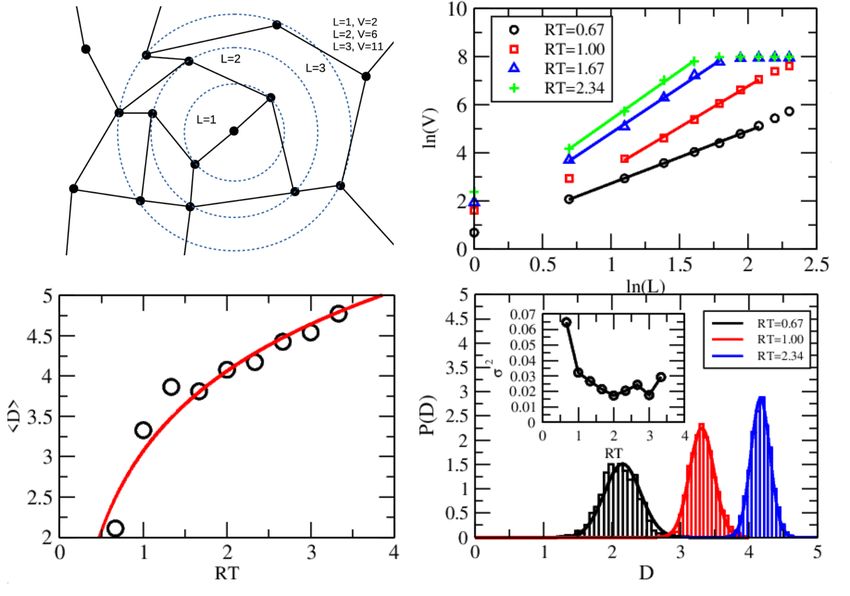
quantum and other phases phenomena emerging in many-body systems[15, 16, 17], that could be also
relevant to emergent spacetime and its dimensionality, through entanglement[15].
    In this paper we consider spatio-dimensionless physical systems, modelled via the most structureless
models, random networks[18, 19], which are discrete mathematical models that do not inherently have
a fixed spatial dimension. We consider uniform networks and study their quantum statistical electronic
properties, using tools like the density of states(DOS) and the inverse participatio ratio(IPR). We find
that for small ratio of edges over vertices in the network RT its electronic properties resemble those of
graphene/honeycomb lattices with properties like linear dispersion relation at the band center at energy
E=0 and edge states concentrated at the spatial boundary of the network [20, 21, 22, 23, 24]. We find
persistent localized states (PLS) at various energies including E=-1,0,1 and others, for example related
to the golden ratio, via the study of the DOS and the IPR. These states comprise primarily of single
unconnected vertices (0D order) at E=0 and one-dimensional(1D) clusters (1D order) for the other
energies, where the wavefunction is localized. The energy of these 1D ordered states is determined
by the dispersion of 1D tight-binding chains formed by the 1D clusters of various lengths. The 0D
ordered states at E=0 spread over the whole network, while the 1D ordered states are concentrated at
the spatial boundary of the network, resembling the edge states in confined graphene systems with zig-
zag edges[20, 21, 24]. As the number of edges between the vertices in the network increases, the DOS
approaches the Wigner semicircle, corresponding to ensembles or random symmetric matrices, and the
number of PLS is gradually reduced until they disappear for large RT . Finally we calculate the spatial
dimension D of the networks, i.e. the dimension of the manifold in which they can be embedded. We
find that the networks which resemble graphene have D ≈ 2, fitting into a 2D plane. The dimension
is increased logarithmically as RT increases and the network becomes more dense as more edges are
added between its vertices. Additionally D reaches integer values like D ≈ 4 apart from non-integer
ones. Our results show that universal phenomena can manifest in physical systems irrespectively of their
spatial dimension. In addition we briefly discuss the relation of our results to emergent spacetime and
relativity/gravity from discrete mathematical models.

2. Network model
Random networks are discrete mathematical models comprising of many vertices randomly connected
with edges[18, 19]. They can be used to express relations between different quantities, which is
useful for example in simulating various real world behaviors such as propagation of behavioral
patterns in social networks or in communications technology. Random networks are also useful in
studying various localization phenomena in mesoscopic and random waveguide systems, theoretically
and experimentally[25]. The probability distribution of the number of edges at each vertex (degree deg)
determines the type of network. In the current paper we choose the most simple type, uniform networks
whose degree at each vertex follows a box distribution. Essentially we have a fixed number of vertices n
and edges m between them randomly distributed forming a random network G(n, m). All configurations
                                                     n
of the edges among the vertices, whose number is (m   2 ) , have an equal probability to appear. The mean

degree for each vertex in the uniform network is given by < deg >= 2 m      n which can be interpreted as
the average connectivity in the network. Note, there are no multi-edges or loops namely the network is a
simple undirected graph. We define the ratio of vertices over the edges in the network RT = m     n , which

is half its average connectivity RT = 2 .
    We examine how a quantum particle behaves as it propagates through the tight-binding lattice formed
by the random network. i.e. the electronic properties of the random network. The Hamiltonian of the
system can be written as
                                                m
                                                   (c†i cj + h.c.)
                                               X
                                        H=                                                              (1)

where   c†i (ci )   is the creation(annihilation) operation for a particle at vertex i in the random network.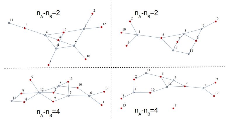
Figure 1. Various random networks for different values of the the ratio between the number of edges over
the number of vertices RT . The number of vertices is n=3000 for all the cases shown. For RT = 0.67
the network is almost planar with few overlapping edges, meaning that it can be fitted approximately into
a 2D plane. As more edges are added RT increases and the network becomes spatially more dense.

The indexes i,j are randomly sampled and create m pairs, representing the edges between the vertices
in the network. The Eq. 1 is a random matrix with a fixed number of elements m (the number of
edges) with the value of one, randomly distributed inside the matrix. In certain cases, such random
network Hamiltonians have been shown to belong to the same universality class as models used to study
Anderson localization phenomena[25]. For example regular tight-binding lattices like the square or the
cubic lattice with a random on-site potential (Anderson model). The randomly distributed elements in
the Hamiltonian matrix Eq. 1 induce interference effects leading to localization of the wavefunctions as
in the Anderson model or in random matrix theory(RMT) models.

3. Energy spectrum
In this section we examine the properties of the energy spectrum of the random networks via the
distribution of eigenvalues of Eq. 1, i.e. the density of states (DOS) of the random network. Firstly
there are two limiting cases worth mentioning. When all the n vertices in the network are disconnected
(m=0) then all the elements of the Hamiltonian Eq. 1 are zero resulting in n zero eigenvalues and a
DOS localized at energy E=0. On the other hand when all the vertices in the network are connected
Figure 2. The distribution of eigenvalues for the networks, i.e. the density of states (DOS) for various
values of the ratio of edges over vertices RT , represented by the black boxes. We have considered
100 different configurations/realizations of the network (runs). The DOS in the upper panels contain
features from graphene/honeycomb lattice systems, as shown from the comparison with the graphene
DOS represented by the blue dashed curve. A linear behavior of the DOS is shown in the insets as
for graphene. As RT increases and the network becomes more dense the DOS starts resembling the
distribution of eigenvalues of random symmetric matrices, the Wigner semi-circle represented by the red
curves. A prominent peak at E=0 is present in all cases coming from many states at this energy persistent
for all networks.

with each other, the Hamiltonian is full apart from its diagonal which has all its elements equal to zero.
In the intermediate case, for an arbitrary number of vertices n and edges m in the network we have
found two major forms for the DOS. The results are shown in Fig. 2. In the plots we have removed
the eigenvalues E=0 coming from disconnected vertices in the network which lead to lines/columns of
zeros in the Hamiltonian.      For low ratio RT in the two upper panels of Fig. 2 the DOS of the
random network resembles that of a graphene/honeycomb lattice as can be seen from the comparison
between the blue dotted line and the histogram. The main features are two peaks at energies E=-1,1
appearing in both cases and a linear dispersion DOS(E) = α|E| near E=0 shown in the insets of the
upper panels. We note that for low RT there is a large probability that the network contains many
disconnected components as shown in Fig. 1. We have found that these components largely contribute
in the number of states appearing at E=-1,1. Another main feature is a peak at E=0 which appears also
for confined graphene systems with zig-zag edges like flakes and nanoribbons, due to edge states at
E=0[20, 21, 24]. We examine the localization properties of these states in the following sections. The
resemblance to graphene can be seen schematically by the network presented in the upper left panel of
Figure 3. The inverse participatio ratio (IPR) for various values of the ratio of the number of edges over
the number of vertices in the network, for 100 runs. The states across the whole energy spectrum become
in average less localized as the network becomes more dense, with increasing RT . Various persistent
localized states (PLS) can be distinguished at various energies including E=-1,0,1 where IPR forms
vertical lines with high values. The number of PLS at E=-1,1 is gradually decreased with increasing RT .

Fig. 1. The network consists primarily of triangles and polygons whose corners consist of vertices that
are connected mostly to three or four neighboring vertices. In addition there are rarely any crossing
edges, i.e. the network is approximately planar, meaning that it can be fitted into a two-dimensional(2D)
plane. This structure is very similar to a graphene/honeycomb lattice which is a 2D plane of hexagons
with every lattice site having three neighboring sites, i.e. the connectivity is three.
   The peaks at E=-1,0,1 and the linear dispersion near E=0, gradually disappear as RT increases as can
be seen in the lower panels of Fig. 2. As more edges are added in the network its Hamiltonian starts to
resemble ensembles of random symmetric matrices whose distribution of eigenvalues follow the Wigner
semicircle, as the size of the matrices approach infinity. The Wigner semicircle function is defined as
                                         2 √
                                           πR2
                                                R2 − x2 −R ≤ x ≤ R
                                f (x) =                                      .                          (2)
                                           0                  otherwise

The above equation for various R is represented by the red continuous curve in Fig. 2 and describes
sufficiently the DOS for the cases shown in the lower panels. Some features of the DOS at its edges are
also captured by the Wigner semicircle in the upper panels for low RT . In overall we see that the DOS
of the random network contains features from both graphene/honeycomb lattices and disordered sytems
described by random symmetric matrices(Hamiltonians). The contribution of these two systems on the
electronic properties of the network depends on the value of RT , which determines the spatial density
Figure 4. Some examples of small networks demonstrating the partial bipartite symmetry. Red vertices
form a sublattice of disconnected vertices (A) while the rest of the vertices form another sublattice (B).
The difference in the number of vertices/sites between the two sublattices nA − nB leads to an equal
number of E=0 states. The wavefunction of these states is zero on the B sublattice which has the least
number of sites.
of the network. Sparse networks for low RT resemble graphene, while dense networks for large RT
resemble disordered systems.
The main difference with regular lattices such as the square, the cubic and the hypercubic is that their
DOS reaches gradually a Gaussian distribution as the lattice connectivity, i.e. the number of neighbors
at each site in the lattice goes to infinity.
4. Localization properties
In Fig. 3 we show the inverse participation ratio (IPR) for the wavefunctions of Eq. 1 defined as
n
X
IP R(E) = |Ψi (E)|4 (3)
i=1
where i runs over the all the vertices and Ψ is the corresponding wavefunction amplitude. We show IPR
for 100 different configurations/realizations of the network (runs). There are two major features that we
can observe. As RT increases and the network becomes spatially more dense, IP R decreases in average.
This means that the corresponding wavefunctions become in average less localized with increasing
RT . We have verified that these wavefunctions corresponding to low values of IP R spread over the
whole network with random amplitudes at each vertex, resembling chaotic wavefunctions encountered
in disordered tight-binding lattices[26, 27]. Another major feature that we can observe in Fig. 3 is
persistent localized states (PLS) appearing at various energies corresponding to high values of IP R,
forming persistent vertical lines for all RT . We can clearly distinguish PLS at energies E=-1,0,1 which
correspond to peaks in the DOS shown in Fig. 2. As shown in the inset of Fig. 3 the number of these
states are reduced as RT increases. We have found that the states at E=0 are localized at vertices along
the whole network which are not connected by edges. All the E=0 states are localized on the same
vertices albeit with different amplitudes. This is one main feature of the E=0 states for all RT and differsFigure 5. Upper left panel: The process of calculating the spatial dimension D of the network by counting how the number of vertices contained into a spherical volume of radius L grows with L. The number of vertices added at each step by increasing L are determined by the edges/connections between the vertices. Upper right panel: The linear scaling of ln(V) with ln(L) gives the value of the dimension D from the relation V ≈ LD . Lower left panel: The mean value of D (open circles) for 1000 configurations/realizations (runs) of the network versus the ratio RT. Integer and non-integer values like D ≈ 4 are reached. The dimension follows a logarithmic behavior D ≈ log(RT = 2 ) represented by the fitting red curve, as for regular lattices of integer dimension like the square and the cube. Lower right panel: The propability distribution of D follows the normal (Gaussian) distribution whose variance is decreased with increasing RT as shown in the inset. from confined graphene systems with zig-zag edges which contain edge states at E=0 concentrated at the boundary of the system [20, 21, 24]. We can consider that the PLS at E=0 in the network, form a quantum phase of zero-dimensional (0D) order, since the wavefunction lies only on disconnected vertices. On the other hand we have found that the PLS at E=-1,1 are concentrated only at the spatial boundary of the network and localize mostly on pairs of vertices connected with an edge (bonds). This bond-ordered localized phase disappears for large RT indicating a phase transition at some critical value of RT . On the other hand the E=0 states persist even for large RT as shown by the peaks in the DOS in Fig. 2. Other√ cases of PLS appear also at other energies for example at E = −φ, −1 + φ, 1 − φ, φ where φ = (1+2 5) is the so called golden ratio. The wavefunctions of these states are localized primarily on lines of vertices (1D clusters) with fixed length, for example lines of four vertices for the energies related to the golden ratio, instead of bonds, and disappear for large RT as for the PLS at E=-1,1. All the phases expect those at E=0 can be considered as quantum phases of one-dimensional (1D) order. We have found that the energies of these 1D ordered states are coming from tight-binding chains whose length is determined by the length of the 1D clusters contained in the 1D ordered phases. The dispersion of a tight-binding chain
with N sites is given by
                                                 nπ
                                   E = 2 cos          , n = 1, 2, . . . , N.                            (4)
                                               N +1
The networks contain mostly the eigenvalues of the above equation for low N corresponding to short
chains. For example some of the E=-1,1 eigenvalues in the network come from Eq. 4 for N=2(chain with
two sites) and the corresponding wavefunctions are localized along bonds of vertices. The case N=4
gives the energies related to the golden ration. In general, the wavefunctions of the states in the network
coming from Eq. 4 are localized along lines of vertices of length N and lie at the spatial boundary of the
network, connected with one edge to the rest of the vertices, resembling dangling bonds. In this sense
these 1D ordered states at energies coming from Eq. 4 bear similarity to the edge states appearing in
confined graphene systems, like flakes and ribbons, which are concentrated along the zig-zag edges of
these systems[20, 21, 24] and persist even with disorder[27]. Also, a large contribution to the eigenvalues
Eq. 4 comes from disconnected chains in the network of length N.

5. Partial bipartite symmetry
The appearance of the E=0 wavefunctions only on vertices of the network that are not directly connected
with an edge can be explained as a consequence of a partial bipartite symmetry of the random
networks[28, 29, 30]. The random network if seen as a lattice can always be split into two sublattices,
say A and B with nA and nB sublattice sites respectively. Additionally it can always be splitted in such
a way that there are no edges between the sites in one of the sublattices, say A. Then the Hamiltonian of
the system can be simplified if written in the basis of A and B sites, as

                                                    0    HAB
                                          H=        †           .                                     (5)
                                                  HAB    HBB

We can write the Schrodinger difference equations centered on A and B sites as

                                         EΨµA,i = j ΨB,j
                                                   P
                                                                                                         (6)
                                   EΨµB,i = j ΨA,j + k ΨB,k
                                             P           P

                                                                                  P
By setting E=0 we can see that the upper equation in Eq. 6 transforms to j ΨB,j = 0 which is a
set of nA equations with nB unknowns. If nA > nB then this set of equations can only be satisfied
by setting ΨB,j = 0 since there are more equations than unknowns i.e. the system of equations is
overdetermined. Then the amplitudes on A sublattice ΨA,k can be calculated by the lower equation in
Eq. 6, which is a system of nB equations with nA unknowns and gives nA − nB linearly independent
solutions. Consequently if the random network is split in two sublattices A and B, with one of them
having no edges between its vertices, say A, whose number of vertices is larger than the number of
vertices for the other sublattice B, then there will always exist at least nA − nB states at E=0. In addition
the wavefunction of these states will have zero amplitudes on the sublattice with the smallest number
of vertices, sublattice B. We remark that for periodic lattices like the square lattice which satisfy the
full bipartite symmetry the value nA − nB will depend on the shape of the boundary. For example for
a square sample of square lattice we will always have nA − nB = 1[28] whereas in graphene flakes
nA − nB depends on the size of the system[30]. Depending on the network configuration(run) there
exist in general many different choices of the sublatice whose vertices are disconnected, corresponding
to different partial bipartite symmetries. Note that in rare cases and more frequently in small networks
with a low number of vertices and edges, some of equations for the sublattice A might be identical
reducing the total number of equations for A. If the number of these equations becomes smaller than
the number of B sites then the argument presented above breaks down and the wavefunctions spreads
on both sublattices for the E=0 states. Nevertheless the partial bipartite symmetry is present for any
type of random network and will lead to E=0 states with the properties described above in most cases of
networks with low spatial density corresponding to low ratio of edges over vertices RT .
6. Spatial dimension
In this section we examine the spatial dimension of the random networks, i.e. the dimension of the
ambient space in which they can be embedded. This can be achieved by examining how the connected
vertices fill an ambient space of dimension D, which can take integer or non-integer values. One example
of this process can be seen schematically in the upper left panel of Fig. 5. At each step in the scaling
characterized by the linear length scale L we count the number of vertices that are connected directly
with edges to the previous layer with L-1. This number is added in the overall volume V, which counts
the total number of vertices contained in a spherical volume of radius L. Therefore by calculating the
growth of V with L we can calculate the dimension D of the network via
V ∼ LD . (7)
Some results of this process for different RT can be seen in the upper right panel of Fig. 5. In addition in
the lower left panel we plot the average < D > for 1000 runs (configurations/realizations of the random
network). For RT = 0.67 the network is almost planar as D ≈ 2, fitting into a 2D plane. This is one of
the reasons that the sparse networks resemble graphene/honeycomb lattices and have similar electronic
properties, as we have shown in the previous sections by the comparison between the DOS of the two
systems. As the network becomes spatially more dense due to the increased connectivity, D grows
logarithmically with RT represented by the fitting red curve in the lower left panel of Fig. 5. Integer
and non-integer dimensions like D ≈ 2 and D ≈ 4 are reached. However the electronic properties
of the networks, as we have shown in the previous sections, do not resemble the respective regular
lattices of integer dimension D, like hypercubic lattices, whose DOS approaches a Gaussian distribution
as D increases. Instead the DOS of the random networks follows the Wigner semicircle, resembling
disordered systems described by random symmetric Hamiltonians. A logarithmic dependence of the
spatial dimension on the connectivity can be derived for regular lattices like the square and the cubic.
The connectivity deg at each site in these lattices is four(eight) for the square(cube), giving in general a
logarithmic form deg = 2D ⇒ D ∼ log(deg). Our result in the lower left panel of Fig. 5 shows that
this behavior is valid even for non-integer dimensions. Since RT = 2 the dimension of the random
network depends exponentially on its average connectivity at each vertex < deg >, as for the regular
lattices, despite the non-integer dimensions reached by the random networks. In the lower right panel of
Fig. 5 the probability distribution of D is shown along with the variance σ 2 (fluctuations) in the inset. All
the distributions are normal (Gaussian). The fluctuations are reduced as RT increases, corresponding to
higher dimension and spatially denser networks.
7. Emergent spacetime and relativity/gravity
In this section we discuss briefly the relation of our model with the notion of emergent spacetime and
relevant relativistic and gravitational effects. A natural way, in the sense of being the most structureless
lacking an inherent spatial dimension, would be to consider spacetime or space as a collection of random
relations between abstract objects, sometimes called atoms of space[3, 4, 5, 6, 7, 8, 9, 10, 12, 13, 14],
with various constraints. These relations can be naturally modeled by random networks, with the abstract
objects(relations) represented by the vertices(edges), and the constraint in our case being the fixed ratio
defined as the number of edges over the number of vertices RT . Essentially space could be represented
as a quantum mechanical superposition of the different realizations of the random networks for fixed
RT . Then one of the main issues would be if the network can be reduced to a continuous manifold at
a limit of large number of vertices and whether geometry can emerge in such a system. For instance,
when RT = 0.67 in the random network that we studied, its spatial dimension is D ≈ 2 resembling
a 2D plane. Moreover its electronic properties, as indicated by the DOS, resemble those of graphene,
which is a 2D honeycomb lattice with the electrons following the Dirac equation near low energies E=0.
Electrons in graphene behave relativistically as massless particles with the speed of light c being replaced
by the Fermi velocity of the electrons vf , with linear energy dispersion E = vf k. The similarities ofthe electronic properties between graphene and spatially sparse random networks, pose an intringuing
question, whether relativistic effects are also encountered in those random networks. We remark also
that D ≈ 4 is reached at RT=2, when the number of edges is double the number of vertices, which
would be tempting to relate to 4D spacetime in the models describing our universe. We note that time
in network/graph models can be integrated either in the network itself[6, 7, 8] or can be treated as an
external updating rule[9, 10].
In addition gravitational effects could potentially emerge in a random network approach to space.
Various definitions of the curvature at each vertex in the network exist[31, 32, 33, 34, 35], the simplest
one being for tree and grid graphs
deg(i)
K(i) = 1 − . (8)
2
where deg(i) is the number of connected neighbors at vertex i in the network. Moreover the Ricci
curvature tensor can be calculated in graph/network models[31, 33]. In addition geodesics can be defined
in the network as simply the path between two vertices that has the least number of edges. Again
an intriguing question arises, whether the curvature in the network can be related to the Riemannian
curvature used in Einstein’s field equations to describe how the geometry of spacetime, influenced by
the mass-energy distribution, gives rise to gravitational effects. The density of vertices in the network
could represent mass while edges can be related to the energy[9, 10]. In this sense the PLS that we
have found in the networks at various energies, comprising of lines of vertices (1D order), could be
loosely interpreted as emergent particles, whose mass is determined by the number of vertices in these
1D structures.
The general question of how geometry arises from discrete mathematical models is fundamental issue
in both mathematics and physics. Another related problem is how to construct mathematics and physical
theories in non-integer spatial dimensions or in the complete absence of spatial dimensions like the
approach that we follow in the current manuscript, using random networks.
8. Summary and Conclusions
We have studied the quantum statistical electronic properties of random networks which inherently lack
a fixed spatial dimension. We have found that the electronic properties of network contain features
from graphene/honeycomb lattice systems and disordered systems described by random symmetric
Hamiltonians. The similarities to graphene occur for spatially sparse networks with low ratio of edges
over vertices RT and include features like linear energy dispersion relation at the band center at E=0
and various persistent localized states (PLS) concentrating at the spatial boundary of the networks,
resembling the edge states in graphene systems with zig-zag edges. The PLS occur at various energies
for example at E=-1,0,1 and others related for example to the golden ratio, and are localized either at
single unconnected vertices (0D order) or lines of vertices of fixed length which determines their energy
(1D order). As the network becomes spatially more dense its electronic properties, indicated for example
by the DOS start to resemble disordered systems described by random symmetric Hamiltonians whose
distribution of eigenvalues follows the Wigner semi-circle. The PLS apart from those at E=0 gradually
disappear as RT increases and the network becomes more dense, with more edges between its vertices.
Finally we have calculated the dimension D of the ambient space in which the networks can be embedded.
We have found a logarithmic growth of D with RT , reaching integer and non-integer values, implying
an exponential dependence of the average connectivity in the network to D as in regular lattices which
have integer D. In summary we have studied quantum mechanics in physical systems lacking a fixed
spatial dimension, demonstrating various unconventional electronic properties. These properties could
be universal for quantum mechanical systems irrespectively of their spatial dimension. Finally we have
discussed the relation of our results to spacetime and relativistic/gravity effects that could emerge from
discrete mathematical models, like the random networks that we considered.Acknowledgements
We acknowledge resources and financial support provided by the National Center for Theoretical
Sciences of R.O.C. Taiwan and the Department of Physics of Ben-Gurion University of the Negev
in Israel. Also we acknowledge support by the Project HPC-EUROPA3, funded by the EC Research
Innovation Action under the H2020 Programme. In particular, we gratefully acknowledge the computer
resources and technical support provided by ARIS-GRNET and the hospitality of the Department of
Physics at the University of Ioannina in Greece.
References
[1] Mukhi S 2011 Class. Quantum Grav. 28 153001
[2] Dienes K R 1997 Phys. Rept. 287 447 [hepth/9602045]
[3] Rovelli C 2011 Class. Quantum Grav. 28 153002
[4] Rovelli C 2008 Living Rev. Relativ. 11 5
[5] Bombelli L, Lee J, Meyer D and Sorkin R D 1987 Phys. Rev. Lett. 59 521-524.
[6] Dowker F 2014 Annals of the New York Academy of Sciences 1326, 18?25
[7] Dowker F and Zalel S 2017 C R Physique 18:246?253.
[8] Surya S 2019 Living Rev. Rel. 22 5 (2019), arXiv:1903.11544 [gr-qc]
[9] Wolfram S 2020 Complex Systems 29(2) pp. 107?536.
[10] Gorard J 2020 Complex Systems, 29(2) pp. 599?654.
[11] Laughlin R B 2003 Int. J. Mod. Phys. A 18, 831
[12] Lombard J 2017 Phys. Rev. D 95 024001
[13] Verlinde E J 2011 High Energ. Phys. 29
[14] Trugenberger, C.A., J. High Energ. Phys. 2017, 45
[15] Christandl M, Datta N, Ekert A and Landahl A 2004 Phys. Rev. Lett. 92, 187902
[16] Walschaers M, Fernandez-de-Cossio Diaz J, Mulet R and Buchleitner A 2013 Phys. Rev. Lett. 111, 180601
[17] Ortega A, Stegmann T and Benet L 2016 Phys. Rev. E 94, 042102
[18] Newman M E J Networks: An Introduction (Oxford University Press, Oxford, 2010)
[19] Frieze A, Karonski M: Introduction to random graphs. Cambridge University Press (2015)
[20] Nakada K, Fujita M, Dresselhaus G and Dresselhaus M S 1996 Phys. Rev. B 54 17954
[21] Wakabayashi K, Fujita M, Ajiki H and Sigrist M 1999 Phys. Rev. B 59 8271
[22] Novoselov K S et al. 2004 Science 306 666
[23] Geim A K and Novoselov K S 2007 Nature Materials 6 183-191
[24] Heiskanen H P et al 2008 New J. Phys. 10 103015
[25] Zhang Z-Q and Sheng P 1994 Phys. Rev. B 49 83
[26] Amanatidis I and Evangelou S N 2009 Phys. Rev. B 79 205420
[27] Kleftogiannis I and Amanatidis I 2014 Eur. Phys. J. B 87 16
[28] Inui M, Trugman S A and Abrahams E 1994 Phys. Rev.B 49, 3190
[29] Kleftogiannis I and Evangelou S N 2013 arXiv:1304.5968 [cond-mat.dis-nn]
[30] Kleftogiannis I and Amanatidis I 2016 J. Phys.: Condens. Matter 28 045305
[31] Forman R 2003 Discrete Comput. Geom. 29 323
[32] Hoorn P, Cunningham W J, Lippner G, Trugenberger C and Krioukov D 2020 Phys. Rev. Research3 013211
[33] Ollivier Y 2013 In Analysis and Geometry of Metric Measure Spaces. CRM Proc. Lecture Notes 56 197?220. Amer.
Math. Soc., Providence, RI. MR3060504
[34] Samal A et al. 2018 Sci. Rep. 8, 8650.
[35] Knill O 2012 Elemente der Mathematik 67,1, pp1-44 arXiv 1009.2292 2010; Knill O 2011 arXiv 1111.5395You can also read