A STUDY ON PATH LOSS ANALYSIS FOR GSM MOBILE NETWORKS FOR URBAN, RURAL AND SUBURBAN REGIONS OF KARNATAKA STATE
←
→
Page content transcription
If your browser does not render page correctly, please read the page content below
International Journal of Distributed and Parallel Systems (IJDPS) Vol.4, No.1, January 2013

            A STUDY ON PATH LOSS ANALYSIS FOR GSM
            MOBILE NETWORKS FOR URBAN, RURAL AND
            SUBURBAN REGIONS OF KARNATAKA STATE
                                     N. Rakesh 1, Dr.S.K.Srivatsa 2
 1
     Research Scholar, Centre for Research and Development, PRIST University, Tanjore,
                                     Tamil Nadu, India.
                                   sai_rakesh2005@rediffmail.com
      2
          Senior Professor, St. Joseph College of Engineering, Chennai, Tamil Nadu, India.
                                        profsks@rediffmail.com

ABSTRACT
To establish any mobile network system, the basic task is to foresee the coverage of the proposed system in
general. Many such different approaches have been developed, over the past, to predict coverage using
what are known as propagation models. In this paper, measurement based path loss example and
shadowing parameters are applied on path loss models. Here, the measurements are carried out in urban,
rural and suburban areas considering non-line-of-sight terrains with low elevation antennas for the
transceiver (Tx) and receiver (Rx)[5]. The impact of multipath are more emphasized in the rural context.
This causes higher probability of RF signal errors. On the basis of observation and with the help of
clutter, we can present models which give better understanding for urban, rural and suburban regions in
Karnataka state at 940 MHz GSM frequency[5],[26][13].

KEYWORDS
BS, Path Loss, Propagation, Model, GSM.

1. INTRODUCTION
Karnataka state is a tropical region, which comes as southern part of India. The Deccan plateau,
which is not really flat, gradually rises towards the south west. The plateau is still surrounded
with craters in the form of chain of mountains and isolated peaks. Here, rural areas are rich in
green vegetation. Urban areas have moderate climatic atmosphere, with most of the localities in
flat surface terrains and suburban is the combination of the both [5]. GSM (Global System for
Mobile Communications) comes under wireless communication, which depends on the
propagation of waves in the free space and providing transmission of data [13],[21]-[26]. It
extends service by providing mobility for users, which fulfills the subscribers demand at any
terrain covered by wireless network. When we consider the earlier historical legacy, the growth
in mobile communications field has now become less. Here, the paramount factor was to serve
for high quality and high capacity networks. Estimated coverage precisely has become very
pivotal. So, in lieu of accomplishing far more accurate design, coverage of modem cellular
networks and signal strength measurements will be considered as source of data, in order to
provide reliable and efficient coverage locality. This paper focuses on the comparisons between
theoretical and experimental analysis, at channel propagation path loss models at GSM
frequency of 940 MHz, for various terrains in Karnataka state. Here, the clutters show the
vegetation of the different areas for propagation of RF signals [1],[2],[3],[4],[5],[13],[22]-[29].
Figure 1.a. shows the framework of GSM technology.

DOI : 10.5121/ijdps.2013.4105                                                                            53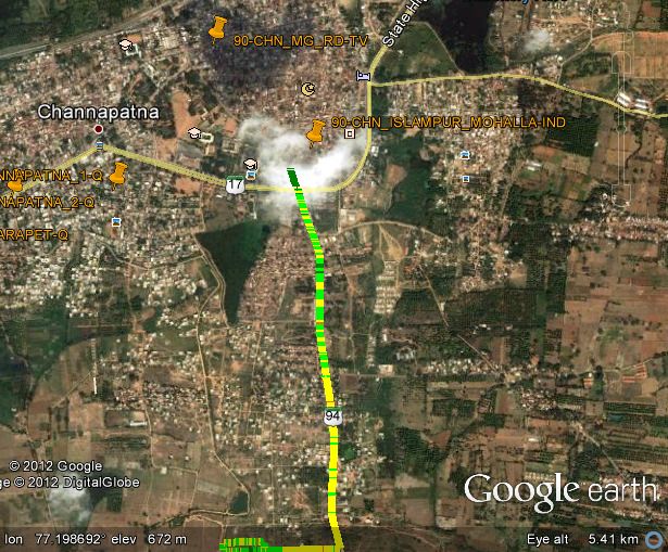
International Journal of Distributed and Parallel Systems (IJDPS) Vol.4, No.1, January 2013

                                    Figure 1.a. GSM framework

2. SIGNIFICANCE OF PROPAGATION FORECAST:
Planning is the key before implementing designs, and also setting up of wireless communication
systems. Precise propagation characteristics of the situation should be known. Usually
propagation provides two types of data, corresponding to the large-scale path loss and small-
scale statistics pertaining to fading issue. Information regarding path-loss is very pivotal, for
knowing the coverage of a base-station (BS) and in tuning it. The statistics provided by the
small-scale parameters pertain only to local field variations. Also in turn this helps to improvise
receiver (Rx) design structure and counter the multipath fading[5],[14],[15]-[34].

3. VARIOUS TYPES PATH-LOSS PREDICTION MODELS
3.1. Empirical Model
It is derived from in-depth field measurements. It is efficient and simple to use. The input data
for the empirical models are generally qualitative, also not very correct, for instance like dense
urban area, rural area and so on [5]-[16].
3.2. Site-specific models
It is based on numerical methods and the finite difference time-domain (FDTD) method. The
input data can be very precise and detailed one [9].
3.3. Theoretical models
It is derived by physical hypothetical assumption, in addition to some moderate conditions. For
instance, when we consider the over-rooftop, diffraction model is derived using physical optics,
assuming constant heights and spacing of buildings [4].
4. DIFFERENT TYPES OF PROPAGATION PATH-LOSS MODELS:
4.1. Cost Hata 231 model
It is recommended for mathematical expression. To calculate the graphical data precisely, its
usage has been put to test at 940 MHz GSM frequency, to foresee the channel path-loss from
source distance d which is the transceiver to the destination receiver antenna upto 5 km;
transmitter antenna height of 60m and receiver antenna height of 3m. To make a study of path-
loss in the GSM frequency range of 940MHz in urban environment, this method is suggested.
    PL = 48.5+35.9log10 (f)-14.84log10 (hb) – ahm + (45.8 – 6.58log10 (hb)) log10d + cm
                                                                                                    54
International Journal of Distributed and Parallel Systems (IJDPS) Vol.4, No.1, January 2013

                                                                                         --(5)
where: d=Distance between transmitter and receiver antenna [km]
f: Frequency [MHz]
hb: Transmitter antenna height [m]
The parameter cm has different values for different environments like 3 dB for urban areas and
the remaining parameter ahm is defined in urban areas as,
                     ahm = 3.25(log10(11.80hr))2- 4.81, for f > 940 MHz
[5]-[19].
4.2. Free space model
It emphasizes on how much strength of signal transmission between transceiver and receiver is
lost.
To calculate the same, we use the following equation:
                        PLFSPL = 32.48 + 20 log10 (d) + 20 log10 (f)

                                                         --(5)
where,
f: Frequency [MHz]
d: Distance between transmitter and receiver [m]
Power is usually expressed in decibels      (dBm)
[5],[6]-[8].
.
4.3. Ericsson model
To predict the path loss, software is provided for network planning engineers developed by
Ericsson company. So, it is called as Ericsson model. The path loss according to this model is
given by the equation:
 PL = a0 + a1.log10 (d) + a2.log10 (hb) + a3.log10 (hb). log10 (d) – 3.3(log10 (11.78hr) 2) + g (f)

                                                        -- (5)
where g(f) is defined as:
g(f) = 44.51log10(f) – 4.79(log10(f))2 )
-- (5)
and
f =Frequency [MHz]
hb=Transmission antenna height [m]
hr=Receiver antenna height [m]
[5],[10],[11]-[25].

4.4. Hata model
It falls under empirical propagation models. It is well suited model for the Ultra High Frequency
(UHF) band. Currently, this model is tested with 940 MHz GSM frequency. Here, empirical
calculation method is applied to predict the model at, frequency range 940 MHz. In this model,
path loss is given by the following equation,
                                              PL = Afs + Abm – Gb - Gr

                                                                          -- (8)
where
Afs=Free space attenuation                     [dB]
Abm= Basic median path loss                    [dB]
Gb= Transmitter antenna height gain factor and
                                                                                                    55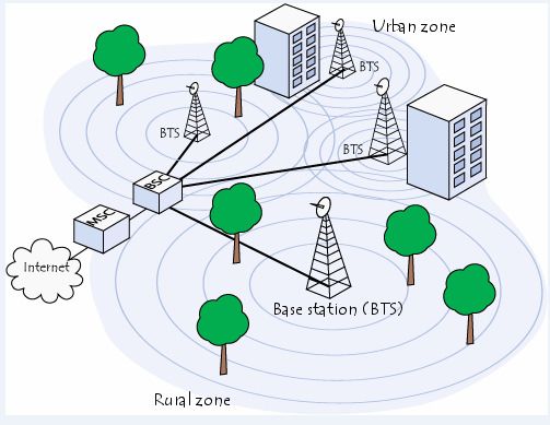
International Journal of Distributed and Parallel Systems (IJDPS) Vol.4, No.1, January 2013

Gr=Receiver antenna height gain factor
These factors can be divided and given by the equation:
Afs = 93.6 + 20log10+20log10 (f)
Abm= 21.41+9.83log10 (d) +8.782log10 (f) + 9.58[log10 (f)] 2
Gb = log10 (hb/200){14.865+ 6.1[log10(d)]2}
When dealing with gain for urban cities, the Gr will be expressed in terms of the following:
                            Gr = [42.58 + 13.7log10 (f)][log10 (hr) – 0.586]

                                                                        -- (8)
For quite large urban areas,
Gr = 0.860hr – 1.960
where,
d= Distance transmitter and receiver antenna in [km]
f= frequency range in [GHz]
hb=Transmitter antenna height in [m]
hr=Receiver antenna height in [m] and
[5],[19],[24],[25],[28]-[35].

4.5. SUI model
This model inherits Hata model’s frequency. Hence it is tested with GSM frequency of 940MHz.
Little bit of correction in parameters, can be extended up to 3 GHz band frequency. In this
model, the BS antenna height can be varied from 10 m to 80 m and at receiver end, the height
can vary between 2 m to 20 m.SUI model comes out with three different types of terrain like
terrain A dense urban locality, terrain B has hilly regions and terrain C for rural with moderate
vegetation. Here, we concentrate on urban path loss with different ranges of receiver antenna
height. The general path loss expression of the SUI model is presented as :
                                      PL = A + 1Oylog10 ( d /d0) + Xf + Xh + s for d > d0

                                                                        -- (5)
where the parameters are as follows,
d= Distance between BS and receiving antenna [ m]
d0= 100 [m]
λ=Wave length [m]
Xf=Correction for frequency 940 [MHz]
Xh=Correction for receiving antenna height          [m]
s= Correction for shadowing                         [dB]
and y=Path loss exponent
By statistical method, the random variables are taken as the path loss exponent y and the weak
fading standard s is derived. The parameter A is defined as,

                                                               ସπୢబ
                                               A = 20log10 ቀ     λ
                                                                    ቁ

                                                                            -- (5)
and the path loss exponent y is given as follows,

                                                                                                    56
International Journal of Distri
Distributed
buted and Parallel Systems (IJDPS) Vol.4, No.1, January 2013
Yy = a – bhb + (c/hb)
Here, the parameter hb is the base station antenna height. This is between 15 m and 90 m range.
The constants a, b, and c depend upon the types of terrain, here our study, urban area. The value
of parameter γ propagation in an urban area,6 < γ < 9 for urban NLOS environment. Th The
frequency correction factor Xf and the correction for antenna receiver height
Xh for the model are expressed as follows,
Xf = 6.2log10 (f/2000)
Xh = -10.9log10 (hr/2000)
[5],[12],[15],[16],[17]-[36].
5. METHODOLOGY USED FOR MEASUREMENT
5.1. Configuration of measurement
Here, the parameter consisted of constant transmitter and a receiver mounted to a car. A dipole
antenna of omnidirectional quarter
quarter-wave
wave with 4 dBi was installed on a tripod and connection is
established to the signal transmitter with a 12 meter feeder cabl
cable.
e. The continuous narrowband
wave signal with GSM frequency of 940 MHz was input given to the Tx antenna with 30 dBm
power capacity. The spectrum analyzer inside the car gives details of the timing intervals for
every one second. Figure 4.1.a. shows the fr framework
amework of the above concept
[9],[10],[11],[21],[22]-[24].
Figure 4.1.a. Measurement framework
57International Journal of Distributed and Parallel Systems (IJDPS) Vol.4, No.1, January 2013
5.2. Environmental measurement
With GSM frequency of 940 MHz RF signal, measurement were performed during July 2012
and the measurement campaign consisted of three slightly various propagation environments in
MG Road,Bangalore,Karnataka,India;Channapatna, Karnataka,India;Kannaswadi, Karnataka,
India. The field measurement survey was performed in Kannaswadi district reflecting a typical
suburban region. The second measurement survey was performed in Bangalore district reflecting
a typical urban region and the third measurement survey was performed in Channapatna district
reflecting a typical rural region.
Typical urban region comprises of blocks of densely constructed buildings. In general, an
average building height is more than 20 meters and buildings may have ten to fifteen floors. In
conjunction, the region is surrounded by parks and open parking areas. Typically 25% of the
area is filled with buildings built of concrete blocks. In rural region with thick vegetation of
highly raised trees, some sequence of houses built with huts; and some part of the place with
concreted buildings. Around 45% of the area filled with more huts, in contrast with suburban,
which is combination of both counterparts [21],[26],[27],[30],[31].
6. AERIAL VIEW OF THE CLUTTER SHOWING VARIOUS TERRAINS
6. Table gives legends of different variations
Figure 6.a. shows the clutter of propagation signal in urban terrain of MG Road.
Figure 6.a. MG Road, Bangalore, Karnataka, India
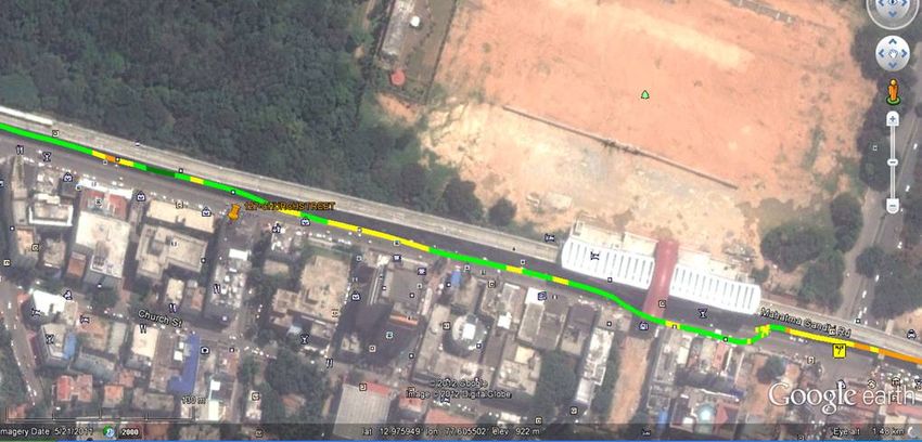
Figure 6.b. shows the clutter of propagation signal in rural terrain of Channapatna.
58International Journal of Distributed and Parallel Systems (IJDPS) Vol.4, No.1, January 2013
Figure 6.b. Channapatna, Karnataka, India
Figure 6.c. shows the clutter of propagation signal in suburban terrain of Kannaswadi.
Figure 6.c. Kannaswadi, Karnataka, India
7. EQUIPMENT AND MEASUREMENT DETAILS DEPLOYED
To measure, we applied a drive test to measure in the location for which a path loss model is to
be designed. Table 7.a. shows the equipment and data used for field measurement in urban area
as follows.
59International Journal of Distributed and Parallel Systems (IJDPS) Vol.4, No.1, January 2013
Table 7.a. Measurement details for path loss at MG Road
Antenna Andrews
Model 65/6deg tilt
Gain 17 dbi
Mobile used C5/antenna 7 dbi
Distance in km Rx level in dBm Tx power in dBM Attenuation in dB
280 -65 43 22
400 -75 43 32
500 -85 43 42
800 -95 43 52
Table 7.b. shows the equipment and data used for field measurement in rural area as follows.
Table 7.b. Measurement details for path loss at Channapatna
Antenna Andrews
Model 65/6deg tilt
Gain 17 dbi
Mobile used C5/antenna 7 dbi
Distance in km Rx level in dBm Tx power in dBM Attenuation in dB
150 -65 43 22
190 -65 43 22
200 -65 43 22
500 -65 to -75 43 32
1000 -75 to -85 43 42
Table 7.c. shows the equipment and data used for field measurement in suburban area.
Table 7.c. Measurement details for path loss at Kannaswadi
Antenna Andrews
Model 65/6deg tilt
Gain 17 dbi
Mobile used C5/antenna 7 dbi
Distance in km Rx level in dBm Tx power in dBM Attenuation in dB
100 -65 43 22
190 -65 43 22
200 -65 43 22
800 -65 to -75 43 32
1800 -75 to -85 43 42
60International Journal of Distributed and Parallel Systems (IJDPS) Vol.4, No.1, January 2013
8. SIMULATED RESULTS OF VARIOUS TERRAINS
The simulated output in Figure 8.a. generated shows the various model path losses in urban
areas.
Figure 8.a. Path loss at MG road urban at 940 MHz GSM frequency
The simulated output in Figure 8.b. generated shows the various model path losses in rural areas.
Figure 8.b. Path loss at Channapatna rural at 940 MHz GSM frequency
61International Journal of Distributed and Parallel Systems (IJDPS) Vol.4, No.1, January 2013
The simulated output in Figure 8.c. generated shows the various model path losses in suburban
areas.
Figure 8.c. . Path loss at Kannaswadi suburban at 940 MHz GSM frequency
9. ANALYSIS OF SIMULATED RESULTS OF VARIOUS TERRAINS
The analysis in Figure 9.a. shows the transceiver Tx, receiver Rx and path loss in urban area of
MG road.
Figure 9.a Analysis of path loss at urban area
62International Journal of Distributed and Parallel Systems (IJDPS) Vol.4, No.1, January 2013
The analysis in Figure 9.b. shows the transceiver Tx, receiver Rx and path losses in rural area of
Channapatna.
Figure 9.b. Analysis of path loss at rural area
The analysis in Figure 9.c. shows the transceiver Tx, receiver Rx and path loss in suburban area
Kannaswadi.
Figure 9.c. Analysis of path loss at suburban area
63International Journal of Distributed and Parallel Systems (IJDPS) Vol.4, No.1, January 2013
10. CONCLUSIONS
This work focuses on the path losses of various propagation models. For this, we have chosen
three different terrains of Karnataka state like urban (MG Road), rural (Channapatna) and
suburban (Kannaswadi). Here, we used drive test for achieving the same. With the help of
spectrum analyzer and digital capture map tool, we were able to measure the path loss of various
terrain regions and clutter of the same. To the measure the path loss between Tx and Rx, the RF
range used was 940 MHz GSM frequency. Free space model path loss is less compared to other
with 85 dB in urban, 102 dB in rural and 89 dB in suburban. Hata model is at larger scale with
158 dB in urban area, 139 dB in rural area and 142 dB in suburban area. The SUI model is
maximum in scale in case of rural environment. Further, the work is focused on to test with
Wimax frequency of these terrains.
ACKNOWLEDGMENT
Authors would like to thank Mr.Srinivasan .A, NWS-RF Planning of IDEA cellular Ltd for
providing the measurement equipment and guiding us to implement the concept successfully.
REFERENCES
[1] N.Rakesh and Dr.S.K. Srivatsa,”VoIP: An Overview and Security Aspects”, International Journal of
Computational Intelligence and Information Security, Vol. 1 No. 9, November 2010,pp-66-69.
[2] N.Rakesh and Dr.S.K. Srivatsa,”Imparting Tutorials using online E-Commerce Application and
Virtualization concept of Standalone PC Environment”, Journal of Emerging Trends in
Computing and Information Sciences, Vol. 2, No. 9, September 2011, pp-427 – 439.
[3] N.Rakesh and Dr.S.K.Srivatsa,” A Study on Diverse Communication Protocols”, International Journal
of Computational Intelligence and Information Security, August 2011 Vol. 2, pp – 143-153.
[4] N.Rakesh and Dr.S.K.Srivatsa,” A Comprehensive investigation on SIP Protocol”, CiiT International
Journal of Networking and Communication Engineering, Vol 3, No.9, July 2011, pp – 593-597.
[5] N. Rakesh and Dr.S.K. Srivatsa ,” An Investigation on Propagation Path Loss in Urban Environments
for Various Models at Transmitter Antenna Height of 50 m and Receiver Antenna Heights of 10
m, 15 m and 20 m respective”” International Journal of Research and Reviews in Computer
Science “, Vol. 3, No. 4, pp. 1761-1767, August 2012.
[6] S. R. Saunders M. Hata, Empirical Formula for Propagation Loss in Land Mobile Radio Services,
IEEETransactions on Vehicular Technology, Vol. VT 29 August 1980, pp. 317-325.
[7] Z. Nadir, N. Elfadhil, and F. Touati , Pathloss determination using Okumura-Hata model and spline
interpolation for missing data for Oman World Congress on Engineering, IAENG-WCE-2008,
Imperial College, London, United Kingdom, 2-4 July,2008, pp.422-425.
[8] M. Hata, “Empirical formula for propagation loss in land mobile radio services,” IEEE Trans. Veh.
Technol., vol. VT-29, pp. 317–325, Aug. 1980.
[9] S. Y. Seidel and T. S. Rappaport, “Site-specific propagation prediction for wireless in-building
personal communication system design,” IEEETrans. Veh. Technol., vol. 43, pp. 879–891, Nov.
1994.
[10] P. E. Morgensen, P. Eggers, C. Jensen and J. B. Andersen , ”Urban Area Radio Propagation
Measurements at 955 and 1845 MHz for Small and Micro Cells”, IEEE GLOBECOM ’91, 1991.
[11] K. L. Blackard, M. J. Feuerstein, T. S. Rappaport, S. Y. Seidel S and H. H. Xia, “Path loss and delay
spread models as functions of antenna height for microcellular system design", IEEE 42nd
Vehicular Technology Conference, 1992.
[12] Sharma K, and Singh K., “Comparative Analysis of Propagation Path loss Models with Field
Measured Data,” International Journal of Engineering Science and Technology, Vol. 2, pp. 2008-
2010, 2010.
64International Journal of Distributed and Parallel Systems (IJDPS) Vol.4, No.1, January 2013
[13] Gordon L. Stüber, (2002). Principles of Mobile Communication. USA:Kluwer Academic Publishers.
[14] Faruque, Saleh, (1996) “Propagation Prediction Based on Environmental Classification and Fuzzy
Logic Approximation”, Proc.IEEE ICC‟96, pp 272-276.
[15]Wu, J. and Yuan, D., (1998) “Propagation Measurements and Modeling in Jinan City”, IEEE
International Symposium on Personal,Indoor and Mobile Radio Communications, Boston, MA,
USA, Vol. 3,pp. 1157-1159.
[16] Azubogu, A.C.O et al. (2010) “Empirical-Statistical Propagation Pathloss Model for Suburban
environment of Nigeria at 800MHz band”, The IUP Journal of Science and Technology,
India,pp-45-54.
[17] Moinuddin A .A. and Singh S, “Accurate Path Loss Prediction in Wireless Environment”,
Insttitution of Engineers (India),Vol 88,July 2007, pp. 09 – 13.
[18] Iskander M. and Yun Z., “Propagation Prediction Models for Wireless Communication Systems”,
IEEE Trans on microwave theory and Techniques, Vol. 50, No. 3, March 2002,pp-662-673.
[19] Nadir Z., Elfadhil, N. and Touati, F., (2008) “Pathloss Determination Using Okumura-Hata Model
and Spline Interpolation for Missing Data for Oman Proceedings of the World Congress on
Engineering” Vol I WCE 2008, July 2008, London, U.K,pp-2-4.
[20] Well known propagation model,
[Online].available:http://en.wikipedia.org/wiki/Radio_propagation_model [Accessed: April 11,
2009].
[21] Shalangwa, D. A. and Singh, K. S. (2010). Measurement and Modeling of path loss for GSM 900 in
Sub Urban Environment over irregular terrain. Journal Computer Science and Network Security.
10(8): pp-268 – 274.
[22] Yu – Huei, T. Wen – Shyang, H. and Ce – Kuen, S. (2009), “The influence of propagation in a live
GSM network”, Journal of electrical engineering.7 (1) pp 1 – 7.
[23] Josiane, C. R., Simone, G. C. F., Herminio, S. G and Gervasio P. S. C. (2009). “Path loss model for
densely Arboreous Citie in Amazon region”: pp-1- 3.
[24] J. G. Andrews, A. Ghosh, and R. Muhamed. Fundamentals of WiMAX Understanding Broadband
Wireless Networking. Prentice Hall.edition-2007.
[25] V. Erceg, L. J. Greenstein, S. Y. Tjandra, S. R. Parkoff, A. Gupta, B. Kulic, A.A. Julius and R.
Bianchi, “An Empirically Based Path Loss Model for Wireless Channels in Suburban
Environments”, IEEE Journal on Selected Areas in Communications, Vol. 17, pp. 1205-1211,
July 1999.
[26]Weather.uk.msn.com/region.aspx?wealocations=Karnataka
[27] Adebayo, A. A. (2004). “Mubi region a Geographical synthesis”, 1st edition Paraclete Publishers Ltd,
Nigeria. pp. 23 – 27
[28] Y Okumura, “Field Strength and Its Variability In UHF And VHF Land Mobile Radio Service”
,Review Of Electrical Communication Laboratory, 1968 P16.
[29] W.C.Y.Lee, “Mobile Communication Design Fundamentals”, (2nd Ed), John Wilely&Sons, New
York, 1993.
[30] V. Armoogum, K.M.S. Soyjaudah, N. Mohamudally, and T. Fogarty “Path Loss Analysis between
the north and the south of Mauritius with some Existing Models for Digital Television
Broadcasting for Summer Season at UHF Bands”, Proceedings of the 8th IEEE AFRICON 2007
–ISBN 0-7803-8606-X.X.
[31] A. Arrinda, M. Ma Velez, P. Angueira, D. de la Vega, and J. L. Ordiales,“Local-Area Field Strength
Variation Measurements Of The Digital Terrestrial Television Signal (COFDM 8k) In Suburban
Environments”,IEEE Transactions On Broadcasting, Vol. 45, No. 4, pp. 386-391,(1999).
[32] J.D. Parsons and M.F. Ibrahim, “Signal strength prediction in built-up areas—Part 2: Signal
variability”, IEE Proc., Vol. 130, No. 5, 1983, pp.385–391.
65International Journal of Distri
Distributed
buted and Parallel Systems (IJDPS) Vol.4, No.1, January 2013
[33] F. Ikegami, S. Yoshida, T. Takeuchi, and M. Umehira, “Prop
“Propagation
agation factors controlling mean field
strength on urban streets”, IEEE Trans.Ant. Prop., Vol. 32 (no issue number), 1984, pp. 822
822–829.
[34] J. Walfisch and H. L. Bertoni, “A Theoretical Model of UHF Propagation in Urban Environments”,
IEEE Transactions On Antennas And Propagation, Vol. 36, No. 12, pp. 1788-1796,
1788 1796, 1988.
[35] C. Perez-Vega
Vega and J.M. Zamanillo, “Path Loss Model for Broadcasting Applications and Outdoor
Communication Systems in the VHF and UHF Bands”, IEEE Transactions On Broadcasting,
Vol. 48, No. 2, pp. 91-96,2002.
96,2002.
Authors
Mr.N.Rakesh is a PhD Student in Computer Science and Engineering at PRIST
University,Thanjavur,Tamilnadu.Currently
Currently he is working as Assistant Professor in
Department of Information Science and Engineering at KNS Institute of
Technology, Bangalore. He received the B.E in Information Scien Science and
Engineering degree from Visvesvaraya Technological University Belgaum,
Karnataka
arnataka and M.Tech in Computer Science and Engineering degree from
Dr.M.G.R.University, Chennai in 2005 and 2007 respectively. Subsequently
completed M.B.A in Systems from Alagappa University, Karaikudi, Tamilnadu
andd M.Sc in Computer Science from Alagappa University, Karaikudi, Tamilnadu in 2009 and 2011
respectively. He is having 7 years of experience in academics and published papers in international
journals, also is a member of CSI. His current research activities pertain to VOIP, ATM, Frame Relays,
Network Security, Information Security, Wireless sensor
se Network and topics related to Networks.
Dr.S.K.Srivatsa received the B.E from Jadavpur University in 1968. He received the
M.E and PhD degree from IISc Bangalore in 1972 and 1976 respectively. He retired
as a Professor of Electronics and CCommunication Engineering, Anna University in
2005. Since then, he is a senior
nior Professor in St.Joseph Engineering college, Chennai,
India. He has produced 40 PhD’s and he is the author of well over 500 publications
in reputed Journals and Conference Proceedings. He is a Life Fellow/Life member
in about two dozen professional soc societies. He is the recipient of about a dozen
awards. His areas of interest include Logic design, graph algorithms, networks, image processing and
robotics.
66You can also read