Hybrid calibration procedure for fringe projection profilometry based on stereo-vision and polynomial fitting
←
→
Page content transcription
If your browser does not render page correctly, please read the page content below
Research Article                                                                                                            Applied Optics   1

                                                  Hybrid calibration procedure for fringe projection
                                                  profilometry based on stereo-vision and polynomial
                                                  fitting
                                                  R AÚL VARGAS1 , A NDRES G. M ARRUGO *1 , S ONG Z HANG2 ,                                AND      L ENNY A. R OMERO3
arXiv:2003.04168v1 [physics.ins-det] 9 Mar 2020

                                                  1 Facultad de Ingeniería, Universidad Tecnológica de Bolívar, Cartagena, Colombia
                                                  2 School of Mechanical Engineering, Purdue University, West Lafayette, IN 47907, United States
                                                  3 Facultad de Ciencias Básicas, Universidad Tecnológica de Bolívar, Cartagena, Colombia
                                                  * Corresponding author: agmarrugo@utb.edu.co

                                                  Compiled March 10, 2020

                                                         The key to accurate 3D shape measurement in Fringe Projection Profilometry (FPP) is the proper calibra-
                                                         tion of the measurement system. Current calibration techniques rely on phase-coordinate mapping (PCM)
                                                         or back-projection stereo-vision (SV) methods. PCM methods are cumbersome to implement as they re-
                                                         quire precise positioning of the calibration target relative to the FPP system but produce highly accurate
                                                         measurements within the calibration volume. SV methods generally do not achieve the same accuracy
                                                         level. However, the calibration is more flexible in that the calibration target can be arbitrarily positioned.
                                                         In this work, we propose a hybrid calibration method that leverages the SV calibration approach using a
                                                         PCM method to achieve higher accuracy. The method has the flexibility of SV methods, is robust to lens
                                                         distortions, and has a simple relation between the recovered phase and the metric coordinates. Experi-
                                                         mental results show that the proposed Hybrid method outperforms the SV method in terms of accuracy
                                                         and reconstruction time due to its low computational complexity. © 2020 Optical Society of America
                                                         http://dx.doi.org/10.1364/ao.XX.XXXXXX

                                                  1. INTRODUCTION                                                                 quisition time by requiring a large number of images or require
                                                                                                                                  costly correspondence search algorithms. Other methods con-
                                                  Accurate 3D shape measurement with Fringe Projection Pro-
                                                                                                                                  sist of digitally pre-deforming the fringe pattern to obtain a
                                                  filometry (FPP) requires proper calibration [1–3]. Currently,
                                                                                                                                  distortion-free projected pattern [19, 20]. Nevertheless, the cal-
                                                  most calibration procedures in FPP rely on phase-coordinate
                                                                                                                                  ibration procedure can become elaborate, which decreases the
                                                  mapping (PCM) or stereo vision (SV) methods [4–6]. PCM tech-
                                                                                                                                  flexibility of the calibration procedure.
                                                  niques relate experimental XYZ metric coordinates to phase
                                                  values using polynomial [7, 8] or rational [9–11] fitting func-                    In recent years, a different approach has emerged. Mainly,
                                                  tions. However, they require the use of 2D or 3D targets with                   to combine PCM and SV models to obtain a flexible calibration
                                                  well-known dimensions, and positioning them at distances and                    procedure and a simpler calibration model [21]. For instance, the
                                                  orientations with high precision [12]. Though accurate, these re-               SV calibration parameters were used to fit a polynomial PCM
                                                  quirements lead to expensive calibration experimental setups [1].               model, and such PCM model achieved the same accuracy as
                                                      Alternatively, the extensively adopted SV method provides                   the SV model, but with higher computational efficiency [4, 22].
                                                  much more flexibility by calibrating the projector in a similar                 Therefore, the question becomes, is it possible to use a PCM
                                                  manner as a camera [13]. Hence, the FPP system can be modeled                   model to achieve higher accuracy?
                                                  using the well-established camera calibration methods [14]. The                    To address the above question, we propose a four-stage hy-
                                                  calibration process can be carried out using arbitrarily placed 2D              brid calibration procedure. 1) we carry out a conventional SV
                                                  targets, resulting in a more flexible calibration procedure [15].               calibration of the FPP system considering camera and projector
                                                  However, it is known that lens distortions introduce significant                lens distortions; 2) we obtain the pose of a flat board using the
                                                  errors in the SV model 3D reconstruction [6, 16]. Several strate-               SV model 3) we compute pixel-wise error maps to ideal planes,
                                                  gies have been proposed to compensate for the projector and                     4) we obtain new pixel-wise relationship between (X̂, Ŷ, and Ẑ)
                                                  camera lens distortions to improve accuracy. Some consist of                    and phase values through pixel-wise polynomial fitting. We will
                                                  projecting additional patterns to obtain a direct camera-projector              demonstrate that our approach improves the overall accuracy
                                                  pixel correspondence [17, 18]. Although, they increase the ac-                  while maintaining a low computational complexity.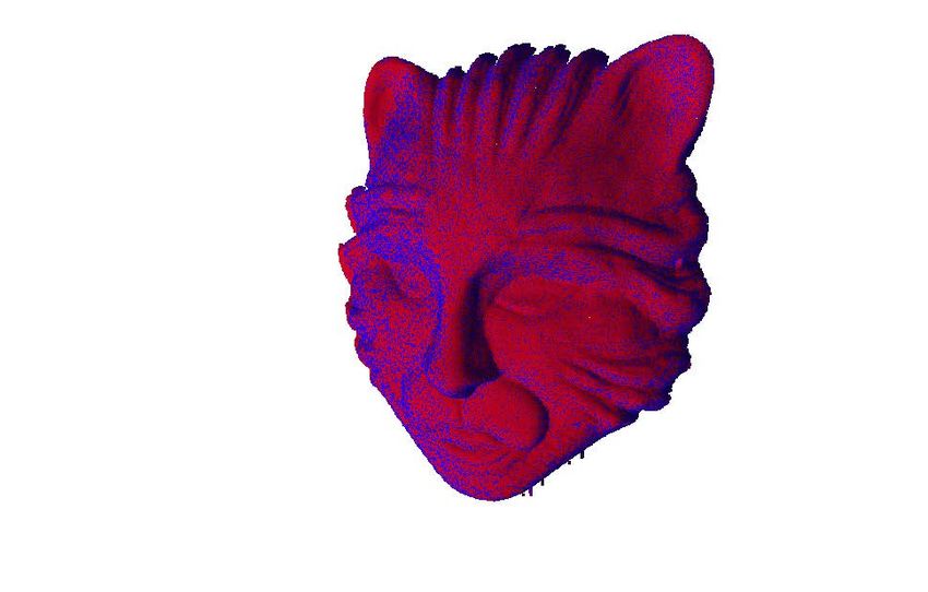
Research Article Applied Optics 2
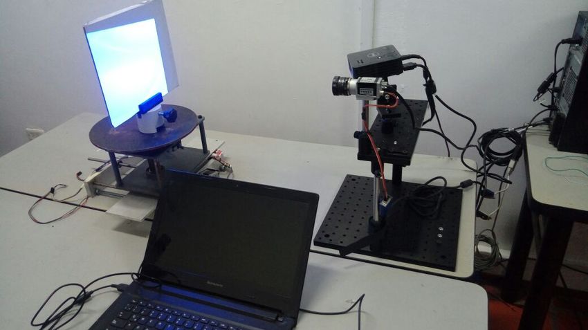
Fig. 1. (a) Experimental Setup. (b) Stereo model diagram of a camera-projector system.
2. METHOD AND MATERIALS The camera and projector distortion lens are modeled as [23]
A. Experimental setup
ud u
=(1 + k1 rn2 + k2 rn4 + k3 rn6 ) n +
In Fig. 1(a), we show the experimental setup, which consists of a
monochromatic CMOS camera Basler Ace-1600gm with resolu- vd vn
tion of 1600x1200 at 60 fps with a focal length of 12 mm at F1.8
2p u v + p2 (rn2 + 2u2n )
(Edmund Optics-58001), a DLP projector DELL M115HD with 1 n n , (3)
native resolution of 1280x800, a checkerboard for calibration 2p2 un vn + p1 (rn2 + 2v2n )
with 8 × 8 mm squares, and a PC workstation. To synchronize
the camera and DLP projector, we duplicate the VGA signal from with
the computer using a VGA splitter and connecting the vertical
sync pulse to the hardware trigger pin of the camera. rn2 = u2n + v2n , (4)
where [k1 , k2 , k3 ] and [ p1 , p2 ] are the radial and tangential dis-
B. Stereo vision calibration tortion coefficients, respectively; [ud , vd ]t and [un , vn ]t refer to
normalized coordinate before and after the distortion correction.
In this work, we begin from the stereo calibration method pro-
To obtain the stereo parameters that describe our system, we
posed by Zhang and Huang [13] to develop a flexible and robust
use a standard stereo calibration procedure using a black and
system calibration approach. The camera-projector system is
white (B&W) checkerboard. We placed the board at 15 different
considered as a binocular framework by regarding the projector
distances and orientations from the system, as shown in Fig 2(a).
as an inverse camera. In Fig. 1(b), we show a schematic of the
In each position, we captured the images shown in Fig. 2(b)-(f).
fringe projection system. Considering a point ( x w , yw , zw ) in the
Using the vertical (Fig. 2(b)) and horizontal (Fig. 2(c)) fringe
world coordinate system (WCS), we find its corresponding co-
images, we recovered the discontinuous phase employing the
ordinate in the camera or projector systems using the following
phase-shifting algorithm with 8 images. Afterward, we apply a
equation,
phase unwrapping algorithm using a centerline image (Fig. 2(d)
xw and Fig. 2(e)) to obtain the absolute phase maps in the horizontal
u f u γ cu
w (φh ) and vertical (φv ) directions[13]. Additionally, we capture a
y texture image of the checkerboard projecting white light on it
s v = 0 f v cv Mw w , (1)
z (Fig. 2(f)).
1 0 0 1 We calculated the corners (ûc , ûc ) with subpixel precision
1 using texture images, and corner coordinates in the projector
image plane (û p , û p ) were calculated using phase values in each
where s is the scaling factor; f u and f v denote the effective focal detected corner. To avoid phase errors in the checkerboard cor-
lengths along u and v directions, respectively; (cu , cv ) is the ners, we used only the phase from the white squares (having
coordinate of the principal point; γ is the skew factor of images morphologically eroded boundaries to avoid black-to-white tran-
axes. The matrix Mw represents a rigid transformation from sition), and we interpolate the phase values using a 5th order 2D
the world coordinate system (WCS) to the camera coordinate polynomial function to all pixels following a similar procedure
system (CCS) or the projector coordinate system (PCS). Usually, as described in Ref. [24].
the WCS matches with the CCS and the transformation WCS to Having determined the coordinates (ûc , ûc ) and (û p , û p ), we
PCS is defined as, used the camera calibration toolbox proposed by Bouguet [25] to
p obtain the intrinsic and extrinsic stereo parameters. The obtained
M w = [ R ( θ s ), t s ], (2)
reprojection errors for the camera and the projector are 0.154 and
where R is a rotation 3×3 matrix, ts is a 3×1 translation vector, 0.099, respectively, which are quite small. In Table 1, we show
and θs denotes a 3×1 vector with the Euler angles. the stereo parameters obtained for our system.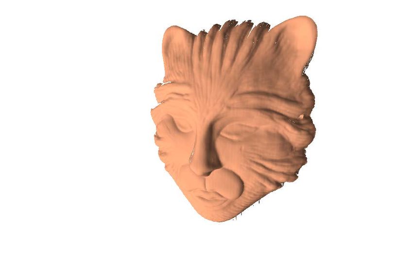
Research Article                                                                                                           Applied Optics     3

Fig. 2. The FPP system is initially calibrated using the conventional (a) Stereo calibration procedure with a B&W checkerboard. It
requires capturing (b)-(f) vertical and horizontal fringe patterns, along with centerline images for absolute phase retrieval, and a
texture image.

Table 1. System stereo parameters of SV calibration.
        Parameter                Camera             Projector
       [cu , cv ] [pix]       794.59, 594.32     632.42, 799.67
       [ f u , f v ] [pix]   2698.42, 2701.55   1949.18, 1953.15
                 γ                 0.84                0.83
              p1                 0.0011               0.0004
              p2                 0.0006               0.0002
              k1                  -0.12               0.002
              k2                  -0.52               -0.077
              k3                   5.08               -0.033
            θs   [◦ ]                 -0.42, 19.08, 0.36
          ts [mm]                  -163.71, -116.73, 135.41             Fig. 3. The hybrid calibration procedure, and the resulting 3D
                                                                        reconstruction method.

C. Hybrid calibration                                                   without the presence of errors caused by intensity variations.
In Fig. 3, we show a block diagram of the proposed hybrid cali-         Although the plane can be placed arbitrarily throughout the
bration procedure. We begin from the standard SV calibration            calibration volume, we decided to manually move the plane in
approach. We then use it to obtain the pose of a flat white board       30 positions using homogeneous displacements. This operation
at different n positions. Suppose that any point (X, Y, Z) of the       guarantees a correct sampling of the region of interest since
3D reconstruction of each pose n, will have small residual er-          fitting a third-order polynomial requires a minimum of four
rors (δx , δy , δz ) relative to the true 3D surface. We assume that    experimental phase-coordinate relations. In each position n,
the best guess to the true surface is an ideal plane estimated          the planes are reconstructed using the SV model, obtaining the
via least-squares. Accordingly, the residual errors are modeled         respective X, Y, and Z coordinates for each camera pixel (uc , vc ).
as the perpendicular distances to that plane. For each recon-
                                                                        C.2. Pixel-wise error function
structed 3D point along the line-of-sight of a given camera pixel
(uc , vc ) we calculate the errors relative to each ideal plane. This   Nevertheless, the SV-reconstructed coordinates have residual
correction does not generally result in a straight line, but in a       errors. To reduce these errors, we fit each reconstructed plane
smooth curve in space. Finally, we use a pixel-wise third-order         to an ideal plane by least-squares. Then, each X, Y, and Z
polynomial regression model to relate the absolute phase values         coordinate of the reconstructed plane is corrected as follows,
to the corrected (X̂, Ŷ, Ẑ) metric coordinates.                                                    X̂ = X − δx ,                            (5)
C.1. Flat board pose estimation                                                                      Ŷ = Y − δy ,                            (6)
The mapping procedure that we propose consists of positioning                                        Ẑ = Z − δz .                            (7)
a flat white board within a predefined calibration volume and
move it through that volume, as shown in Fig. 4(a). We propose          where X̂, Ŷ, and Ẑ represent the corrected coordinates for a
to use a white board since it allows us to have a phase map             camera pixel (uc , vc ), (δx , δy , δz ) are the estimated residual errors
Research Article Applied Optics 4
Fig. 5. A third-degree polynomial function describes suffi-
ciently well the phase φ to ideal (a) X̂, (b) Ŷ and (c) Ẑ coordi-
nates of the image pixel (200, 200). The RMS error maps of
Fig. 4. The (a) Hybrid calibration procedure consists in man-
(d) X̂, (e) Ŷ and (f) Ẑ-calibration show a small error through-
ually displacing a flat white board along a predefined cali-
out most of the field of view.
bration volume. The (b) recovered absolute phase map φ and
metric coordinates (X̂, Ŷ, Ẑ) of an ideal plane estimated for a
position of the flat board are used for the input for the hybrid the X̂, Ŷ and Ẑ corrected experimental data and the fitted poly-
calibration. nomials for each pixel for all poses of the white flat board. In
Figures 5(d)-(f) we show the RMS errors corresponding to φ − X̂,
φ − Ŷ, and φ − Ẑ, respectively. The RMS errors of the polyno-
from the perpendicular distance between the ideal plane and
mial fittings have a maximum of 0.060 mm for the Ẑ coordinate,
each point (X, Y, Z). In Fig. 4(b), we show the phase map using
while for the X̂- and Ŷ- coordinates, the RMS errors are less
vertical fringes and the corrected coordinates for the plane at
than 0.015 mm. Therefore, the third-order polynomial regres-
position n = 15.
sion model correctly describes our system within the calibrated
C.3. Pixel-wise polynomial fit volume, which is approximately 270 mm × 200 mm × 130 mm.
We use a pixel-wise regression model to relate the absolute phase C.4. 3D reconstruction
values to the metric coordinates of the FPP system for each pixel
As shown in Fig. 3, the 3D reconstruction under the proposed
( u c , v c ),
hybrid calibration procedure consists of two stages. First, recov-
X̂ = a3 φ3 + a2 φ2 + a1 φ + a0 , (8) ering the absolute phase per camera pixel from the projected
vertical fringe patterns. Second, evaluating the polynomials
3 2
Ŷ = b3 φ + b2 φ + b1 φ + b0 , (9) from equations Eq. (8)-Eq. (10) to obtain the accuracy-improved
3 2
Ẑ = c3 φ + c2 φ + c1 φ + c0 , (10) 3D reconstruction.
where φ is the absolute phase value for a camera pixel (uc , vc ); 3. EXPERIMENTAL RESULTS
X̂, Ŷ, and Ẑ are the corrected metric coordinates in the camera
coordinate system; and a0−3 , b0−3 and c0−3 are the coefficients of A. Experiment 1: Reconstruction of a flat board
the adjustment polynomials φ − X, φ − Y and φ − Z, respectively. Here, we compare the accuracy of the SV and Hybrid models. To
We have omitted the pixels (uc , vc ) in the notation to avoid do this, we reconstructed a flat white board of 230 mm × 175 mm
making the equations more complicated. positioned within the calibration volume of the hybrid model,
Figures 5(a), (b) and (c) show the experimental data and the and we inclined it relative to the Z axis of the camera, as shown
adjustment polynomial between the phase values and the X̂, Ŷ in Fig. 6(a). This board was reconstructed using the two calibra-
and Ẑ coordinates for the pixel (200, 200) of the camera. Note tion models, and an adjustment to an ideal plane was carried
that the third-order polynomial allows obtaining a correct rep- out by least-squares fitting. In Fig. 6(b), we show the histograms
resentation of the data. We calculate an RMS error between of the plane adjustment error corresponding to each calibrationResearch Article Applied Optics 5
Fig. 6. Experiment 1 results. (a) Flat board. (b) Error histograms
in the reconstruction of a flat board using SV, and hybrid cali- Fig. 7. Experiment 2 results. (a) 3D reconstruction shape of a
bration models. (c) and (d) adjustment error maps of a plane cylinder using the hybrid model. (b) Histogram of Adjustment
reconstructed by SV and hybrid model, respectively. The hy- error of a cylinder reconstructed using the hybrid and SV mod-
brid model significantly improves the accuracy of the 3D re- els. (c) and (d) Error maps of the cylinder reconstructed by SV
construction. model and hybrid model, respectively. The accuracy improve-
ment is also displayed in the 3D reconstruction of a non-flat
object.
model. Note that the hybrid calibration model improves the
accuracy of the reconstruction of the plane, reducing the dis-
persion of the error distribution and obtaining an RMS error of
0.044 mm, which is lower than the RMS error of 0.118 mm ob-
tained with the SV model. Therefore, although the hybrid model
is derived from the SV model, it provides greater precision in
the reconstruction by compensating the residual errors. In the
figures 6(c) and 6(d), we show the error maps obtained with the
SV and the hybrid model, respectively. In Fig. 6(c), we can see
that the residual errors in the SV model vary through the field
of view in a range of [−0.2, 0.2] mm, while the hybrid model has
a more homogeneous error distribution with most errors in the
range of [−0.1, 0.1] mm. Fig. 8. Experiment 3 results. (a) Captured fringe images of a
ceramic mask. (b) 3D reconstruction of the mask. (c) Super-
position of the 3D reconstructions using the hybrid and SV
B. Experiment 2: Reconstruction of a cylinder models.
In this experiment, we evaluate the performance of the pro-
posed calibration model to perform the reconstruction of a non-
flat object, a cylinder. The tested object is a 168mm diameter C. Experiment 3: Complex surface reconstruction
and 215mm height Polyvinyl chloride (PVC) pipe. A section of In this experiment, we performed the reconstruction of a com-
the pipe was reconstructed using the SV and Hybrid models. plex ceramic mask of an approximate size of 160mm×190mm.
Fig. 7(a) shows the 3D shape of the cylindrical cap reconstructed To do this, we projected vertical and horizontal fringe patterns
using the Hybrid model. To assess the shape measurement ca- onto the surface of the object, as shown in Fig. 8(a). It was neces-
pability of each method, we adjust each reconstruction to an sary to project the horizontal strip patterns to compensate the
ideal cylinder by least-squares fitting. The histograms of ad- distortions of the projector in the stereo model, while the hybrid
justment errors obtained for each reconstruction are shown in model only requires the projection of vertical fringes. In Fig. 8(b),
Fig 7(b). Note that the hybrid model allows obtaining a correct we show the reconstruction of the ceramic mask using the hybrid
cylindrical representation of the reconstruction since the errors model. Fig. 8(c) shows the superposition of the reconstructions
are more concentrated around zero, while the histogram of the of the hybrid and SV models. The RMS distance between the
SV model has a higher dispersion. The RMS adjustment errors two reconstructions is 0.075 mm. The reconstruction times of the
obtained with the SV and hybrid models were 0.076 and 0.059 object (683047 points) were 1.04s and 0.14s for the SV models
mm, respectively. Figures 7(c) and (d) show the adjustment error and the hybrid model, respectively.
maps for the SV and hybrid models, respectively. Note that in
the SV model, the largest residual errors are located in the upper D. Experiment 4: Execution time assessment
and lower part of the cylinder; meanwhile, in the error map of Finally, we analyzed the execution times required for the hybrid
the hybrid reconstruction, the errors are uniformly distributed model and the SV model to reconstruct objects of different sizes.
throughout the image. To simulate this, we reconstructed several sections of a studyResearch Article Applied Optics 6
can Optics Meeting (RIAO) in Cancun, Mexico, and at the 2019
SPIE Optical Metrology conference in Munich, Germany [26].
REFERENCES
1. S. Zhang, High-Speed 3D Imaging with Digital Fringe Projection Tech-
niques (CRC Press, 2016).
2. S. Zhang, “High-speed 3D shape measurement with structured light
methods: A review,” Opt. Lasers Eng. 106, 119–131 (2018).
Fig. 9. Experiment 4 results. (a) Reconstructed NxN size win- 3. A. G. Marrugo, J. Pineda, L. A. Romero, R. Vargas, and J. Mene-
dows of an object for reconstruction time analysis. (b) recon- ses, “Fourier transform profilometry in labview,” in Digital Systems,
struction time curves of the SV and hybrid models using (IntechOpen, 2018).
square reconstruction windows with NxN pixels. 4. Z. Cai, X. Liu, A. Li, Q. Tang, X. Peng, and B. Z. Gao, “Phase-3d
mapping method developed from back-projection stereovision model
for fringe projection profilometry,” Opt. Express 25, 1262–1277 (2017).
object with different numbers of pixels. The object of reconstruc- 5. X. Li, Z. Zhang, and C. Yang, “Reconstruction method for fringe pro-
tion is the flat board used in the calibration process, and the jection profilometry based on light beams,” Appl. Opt. 55, 9895–12
reconstruction sections were chosen using square windows with (2016).
a size of NxN pixels, as shown in Fig. 9(a). 6. R. Vargas, A. G. Marrugo, J. Pineda, J. Meneses, and L. A. Romero,
“Camera-projector calibration methods with compensation of geometric
In Fig. 9(b), we show the time required to perform the recon-
distortions in fringe projection profilometry: A comparative study,” Opt.
structions of eight different window sizes using the Hybrid and Pura Apl. 51 (2018).
SV models. Note that the hybrid model performs the 3D recon- 7. M. Vo, Z. Wang, T. Hoang, and D. Nguyen, “Flexible calibration tech-
structions with low computation time compared to the stereo nique for fringe-projection-based three-dimensional imaging,” Opt. Lett.
model. This difference is because the SV model demands sig- 35, 3192–3194 (2010).
nificant time in the compensation of distortions of the projector, 8. J. Huang and Q. Wu, “A new reconstruction method based on fringe
which is carried out with an iterative process. Whereas in the projection of three-dimensional measuring system,” Opt. Lasers Eng.
hybrid model, these distortions are implicitly compensated in 52, 115–122 (2014).
the polynomial model coefficients for each pixel, and no iterative 9. L. Huang, P. S. Chua, and A. Asundi, “Least-squares calibration method
computation is required. for fringe projection profilometry considering camera lens distortion,”
Appl. Opt. 49, 1539–1548 (2010).
10. P. Zhou, X. Liu, and T. Zhu, “Analysis of the relationship between fringe
4. CONCLUSION angle and three-dimensional profilometry system sensitivity,” Appl. Opt.
53, 2929–2935 (2014).
Improving the measurement accuracy of a standard fringe pro- 11. H. Du and Z. Wang, “Three-dimensional shape measurement with an
jection profilometry system typically requires elaborate calibra- arbitrarily arranged fringe projection profilometry system,” Opt. Lett. 32,
tion procedures or sophisticated iterative methods to reduce 2438–2440 (2007).
3D reconstruction error. Here, we have proposed a calibration 12. J. Villa, M. Araiza, D. Alaniz, R. Ivanov, and M. Ortiz, “Transformation
method that leverages the stereo calibration approach for fringe of phase to (x,y,z)-coordinates for the calibration of a fringe projection
projection profilometry and improves the measurement accu- profilometer,” Opt. Lasers Eng. 50, 256–261 (2012).
racy. The hybrid method uses the reconstructions of a flat white 13. S. Zhang and P. S. Huang, “Novel method for structured light system
board as input to obtain pixel-wise polynomials for converting calibration,” Opt. Eng. 45, 083601–083601 (2006).
phase to metric coordinates with higher accuracy than the un- 14. R. Hartley and A. Zisserman, Multiple view geometry in computer
vision (Cambridge university press, 2003).
derlying stereo model. The accuracy improvement was shown
15. Z. Zhang, “A flexible new technique for camera calibration,” IEEE
through several experiments. Moreover, the low computational
Transactions on Pattern Analysis Mach. Intell. 22 (2000).
complexity of the proposed method reduces the execution time 16. R. Vargas, A. G. Marrugo, J. Pineda, J. Meneses, and L. A. Romero,
for 3D reconstruction significantly. “Evaluating the Influence of Camera and Projector Lens Distortion in 3D
Reconstruction Quality for Fringe Projection Profilometry,” in Imaging
FUNDING and Applied Optics 2018, (OSA, Washington, D.C., 2018), p. 3M3G.5.
17. Z. Li, Y. Shi, C. Wang, and Y. Wang, “Accurate calibration method for a
Colciencias (project 538871552485), and Universidad Tecnológica structured light system,” Opt. Eng. 47, 053604–053604 (2008).
de Bolivar (projects C2018P005 and C2018P018). 18. D. Moreno and G. Taubin, “Simple, accurate, and robust projector-
camera calibration,” in 2012 Second International Conference on 3D
Imaging, Modeling, Processing, Visualization & Transmission, (IEEE,
DISCLOSURES 2012), pp. 464–471.
The authors declare no conflicts of interest. 19. K. Li, J. Bu, and D. Zhang, “Lens distortion elimination for improving
measurement accuracy of fringe projection profilometry,” Opt. Lasers
Eng. 85, 53–64 (2016).
ACKNOWLEDGEMENT 20. A. Gonzalez and J. Meneses, “Accurate calibration method for a fringe
projection system by projecting an adaptive fringe pattern,” Appl. Opt.
R. Vargas thanks Universidad Tecnológica de Bolívar (UTB) for
58, 4610–4615 (2019).
a post-graduate scholarship. L.A. Romero and A.G. Marrugo
21. R. Chen, J. Xu, Z. Ye, J. Li, Y. Guan, and K. Chen, “Easy-to-operate
thank UTB for a Research Leave Fellowship. A.G. Marrugo ac- calibration method for structured light systems,” Appl. Opt. 55, 8478–8
knowledges support from the Fulbright Commission in Colom- (2016).
bia and the Colombian Ministry of Education within the frame- 22. Z. Cai, X. Liu, X. Peng, and B. Z. Gao, “Ray calibration and phase
work of the Fulbright Visiting Scholar Program, Cohort 2019- mapping for structured-light-field 3d reconstruction,” Opt. Express 26,
2020. Parts of this work were presented at the 2019 Iberoameri- 7598–7613 (2018).Research Article Applied Optics 7
23. M. N. Vo, Z. Wang, L. Luu, and J. Ma, “Advanced geometric camera
calibration for machine vision,” Opt. Eng. 50, 110503 (2011).
24. X.-L. Zhang, B.-F. Zhang, and Y.-C. Lin, “Accurate phase expansion on
reference planes in grating projection profilometry,” Meas. Sci. Technol.
22, 075301–9 (2011).
25. J.-Y. Bouguet, “Camera calibration toolbox for matlab (2008),” .
26. R. Vargas, A. G. Marrugo, J. Pineda, and L. A. Romero, “A flexible and
simplified calibration procedure for fringe projection profilometry,” in
Modeling Aspects in Optical Metrology VII, , vol. 11057 (SPIE, 2019),
p. 110571R.You can also read