PPL Bench: Evaluation Framework For Probabilistic Programming Languages
←
→
Page content transcription
If your browser does not render page correctly, please read the page content below
PPL Bench: Evaluation Framework For Probabilistic
Programming Languages

SOURABH KULKARNI, KINJAL DIVESH SHAH, NIMAR ARORA, XIAOYAN WANG, YU-
CEN LILY LI, NAZANIN KHOSRAVANI TEHRANI, MICHAEL TINGLEY, DAVID NOURSI,
NARJES TORABI, SEPEHR AKHAVAN MASOULEH, ERIC LIPPERT, and ERIK MEIJER, Face-
book Inc, USA (@fb.com)
We introduce PPL Bench, a new benchmark for evaluating Probabilistic Programming Languages (PPLs) on a
variety of statistical models. The benchmark includes data generation and evaluation code for a number of
models as well as implementations in some common PPLs. All of the benchmark code and PPL implementations
are available on Github. We welcome contributions of new models and PPLs and as well as improvements in
existing PPL implementations. The purpose of the benchmark is two-fold. First, we want researchers as well as
conference reviewers to be able to evaluate improvements in PPLs in a standardized setting. Second, we want
end users to be able to pick the PPL that is most suited for their modeling application. In particular, we are
interested in evaluating the accuracy and speed of convergence of the inferred posterior. Each PPL only needs
to provide posterior samples given a model and observation data. The framework automatically computes and
plots growth in predictive log-likelihood on held out data in addition to reporting other common metrics such
as effective sample size and rˆ.

1   INTRODUCTION
Probabilistic Programming Languages [Ghahramani 2015] allow statisticians to write probability
models in a formal language. These languages usually include a builtin inference algorithm that
allows practitioners to rapidly prototype and deploy new models. More formally, given a model
P(X, Z ) defined over random variables X and Z and given data X = x, the inference problem is
to compute P(Z |X = x). Another variant of this inference problem is to compute the expected
value of some functional f over this posterior, E[f (Z )|X = x]. Most languages provide some
version of Markov Chain Monte Carlo [Brooks et al. 2011] inference. MCMC is a very flexible
inference technique that can conveniently represent high dimensional posterior distributions with
samples Z 1, . . . , Zm that collectively approach the posterior asymptotically with m. Other inference
techniques that are often builtin include Variational Inference [Wainwright et al. 2008], which is
usually asymptotically inexact, and Importance Sampling [Glynn and Iglehart 1989], which is only
applicable to computing an expectation.
   In roughly the last two decades there has been an explosive growth in the number of PPLs.
Starting with BUGS [Spiegelhalter et al. 1996], iBAL [Pfeffer 2001], BLOG [Milch et al. 2005], and
Church [Goodman et al. 2008] in the first decade, and followed by Stan [Carpenter et al. 2017],
Venture [Mansinghka et al. 2014], Gen [Cusumano-Towner and Mansinghka 2018], Turing [Ge
et al. 2018], to name some, in the next decade. Some of these PPLs restrict the range of models they
can handle whereas others are universal languages, i.e, they support any computable probability
distribution. There is a tradeoff between being a universal language and performing fast inference
because if a language only supports select probability distributions, its inference methods can
optimize for that. Different PPLs can be better suited for different use-cases and hence having
a benchmarking framework can prove to be extremely useful. We introduce PPL Bench as a
benchmarking framework for evaluating different PPLs on models. PPL Bench has already been
Authors’ address: Sourabh Kulkarni, skulkarni@umass.edu; Kinjal Divesh Shah, kshah97; Nimar Arora, nimarora; Xiaoyan
Wang, xiaoyan0; Yucen Lily Li, yucenli; Nazanin Khosravani Tehrani, nazaninkt; Michael Tingley, tingley; David Noursi,
dcalifornia; Narjes Torabi, ntorabi; Sepehr Akhavan Masouleh, sepehrakhavan; Eric Lippert, ericlippert; Erik Meijer,
erikm, Facebook Inc, Probability, 1 Hacker Way, Menlo Park, CA, 94025, USA (@fb.com).
Sourabh Kulkarni, Kinjal Divesh Shah, Nimar Arora, Xiaoyan Wang, Yucen Lily Li, Nazanin Khosravani Tehrani, Michael
2                         Tingley, David Noursi, Narjes Torabi, Sepehr Akhavan Masouleh, Eric Lippert, and Erik Meijer

                                        Fig. 1. PPL Bench system overview

used to benchmark a new inference method, Newtonian Monte Carlo [Arora et al. 2019]. In the
rest of this paper, we provide an overview of PPL Bench1 and describe each of the initial statistical
models that are included before concluding.

2   SYSTEM OVERVIEW
PPL Bench is implemented in Python 3 [Team 2019]. It is designed to be modular, which makes it
very easy to add models and PPL implementations to the framework. The typical PPL Bench flow
is as follows:
    • Model Instantiation and Data Generation: All the models in PPL Bench have various
       parameters that need to be specified. A model with all it’s parameters set to certain values is
       referred to as a model instance. We establish a model Pθ (X, Z ) with ground-truth parameter
       distributions(θ ∼ Pϕ ) where ϕ is the hyperprior (a prior distribution from which parameters
       are sampled). In some models theta is sampled from ϕ while in others it can be specified
       by users. PPL Bench is designed to accept parameters at both the PPL level, as well as the
       model level. Therefore, any parameters such as number of samples, number of warmup
       samples, inference method and so on can be configured with ease. Similarly, any model-
       specific hyperparameters can also be passed as input through a JSON file. We can sample
       parameter values form their distributions, which will instantiate the model:
                                                     Z 1 ∼ Pθ (Z )
         We then simulate train and test data as follows:
                                                      iid
                                             X t r ain ∼ Pθ (X |Z = Z 1 )
                                                     iid
                                              X t est ∼ Pθ (X |Z = Z 1 )
      Note that this process of data generation is performed independent of any PPL.
    • PPL Implementation and Posterior Sampling: The training data is passed to various PPL
      implementations which learn a model Pθ (X = X 1, Z ); The output of this learning process
      is obtained in the form of n sets of posterior samples of parameters (one for each sampling
      step).
                                    Z 1...n
                                      ∗
                                            ∼ Pθ (Z |X = X t r ain )
1 Open   Source on Github: https://github.com/facebookresearch/pplbench
PPL Bench: Evaluation Framework For Probabilistic Programming Languages                              3

      The sampling is restricted to a single chain and any form of multi-threading is disabled.
      However, we can run each benchmark multiple times, and we treat each trial as a chain. This
      allows us to calculate metrics such as r hat .
    • Evaluation: Using the test data X t est , posterior samples Z 1...n
                                                                     ∗      and timing information, the
      PPL implementations are evaluated on the following evaluation metrics:
      Plot of the Predictive Log Likelihood w.r.t samples for each implemented PPL: PPL
      Bench automatically generates a plot of predictive log likelihood against samples. This
      provides a visual representation of how fast different PPLs converge to their final predictive
      log likelihood value. This metric has been previously used by [Kucukelbir et al. 2017] to
      compare convergence of different implementations of statistical models.
                                                             n
                                                                                       !
                                                          1Õ
                   Predictive Log Likelihood(n) = log           (P(X t est |Z = Z i ))
                                                                                  ∗
                                                          n i=1
        After computing the predictive log likelihood w.r.t samples over each trial run, the min,
        max and mean values over samples is obtained. These are plotted on a graph for each PPL
        implementation so their convergence behavior can be visualized. This plot is designed to
        capture both the relative performance and accuracy of these implementations.
        Gelman-Rubin convergence statistic r hat : We report r hat for each PPL as a measure of
        convergence by using samples generated across trials. We report this quantity for all queried
        variables.
        Effective sample size ne f f : The samples generated after convergence should ideally be
        independent of each other. In reality, there is non-zero correlation between generated samples;
        any positive correlation reduces the number of effective samples generated. Samples are
        combined across trials and the ne f f as well as nef f /s of each queried variable in each PPL
        implementation is computed.
        Inference time: Runtime is an important consideration for any practical use of probabilistic
        models. The time taken to perform inference in each trial of a PPL is recorded.
   The generated posterior samples and the benchmark configurations such as number of samples,
ground-truth model parameters etc. are stored along with the plot and evaluation metrics listed
above for each run. PPL Bench also allows for model-specific evaluation metrics to be added. Using
the PPL Bench framework, we establish four models to evaluate performance of PPLs:
   (1) Bayesian Logistic Regression model[van Erp and Gelder 2013]
   (2) Robust Regression model with Student-T errors[Gelman et al. 2013]
   (3) Latent Keyphrase Index(LAKI) model, a Noisy-Or Topic Model[Liu et al. 2016]
   (4) Crowdsourced Annotation model, estimating true label of an item given a set of labels
        assigned by imperfect labelers[Passonneau and Carpenter 2014]
These models are chosen to cover a wide area of use cases for probabilistic modeling. Each of these
models is implemented in all or a subset of these PPLs: PyMC3 [Salvatier et al. 2016], JAGS [Plummer
et al. 2003], Stan [Carpenter et al. 2017] and BeanMachine [Tehrani et al. 2020]. The model and PPL
implementation portfolio is expected to be expanded with additional open-source contributions.
Subsequent sections describe these models and implementations in detail along with analysis of
observed results.

3   BAYESIAN LOGISTIC REGRESSION MODEL
Logistic Regression is the one of the simplest models we can benchmark PPLs on. Because its
posterior is log-concave, it is easy for PPLs to converge to the true posterior. For model definition,
see Appendix 8.1. Here, N refers to number of data points and K refers to the number of covariates.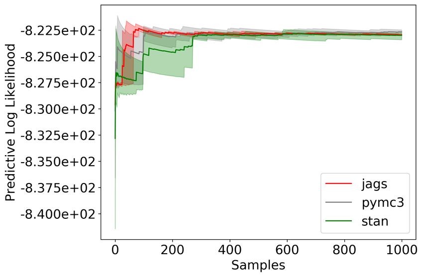
Sourabh Kulkarni, Kinjal Divesh Shah, Nimar Arora, Xiaoyan Wang, Yucen Lily Li, Nazanin Khosravani Tehrani, Michael
4 Tingley, David Noursi, Narjes Torabi, Sepehr Akhavan Masouleh, Eric Lippert, and Erik Meijer
nef f /s nef f /s
PPL N Time(s) PPL N Time(s)
min median max min median max
BeanMachine 20K 298.64 21.74 232.85 416.98 BeanMachine 20K 146.79 3.11 8.48 41.85
Stan 20K 47.06 21.62 25.78 108.63 Stan 20K 35.21 87.71 114.75 361.16
Jags 20K 491.22 0.17 0.18 4.04 Jags 20K 742.40 0.59 1.40 2.87
PyMC3 20K 48.37 23.65 27.10 67.27 PyMC3 20K 45.78 92.50 99.14 137.45
BeanMachine 200K 1167.13 0.003 0.004 0.01 BeanMachine 200K 250.41 1.87 4.00 10.33
Stan 200K 10119.02 0.06 0.06 0.34 Stan 200K 140.58 0.77 1.52 2.40
Table 1. Runtime and ne f f /s for Bayesian Logis- Table 2. Runtime and nef f /s for Robust Regres-
tic Regression. sion
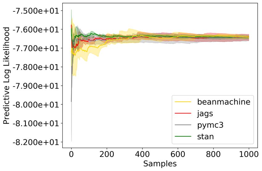
Figure 2 shows the predictive log likelihood for N = 20k and N = 200k. We use half of the data for
inference and the other half for evaluation. We run 1000 warm-up iterations for each of the PPLs
and plot the samples from the next 1000 iterations. We can see from Figure 2 that all the predictive
log likelihood (PLL) of different PPLs converge to around the same value. Thus, in addition to
convergence, the plot could also be used to check the accuracy of the model.
(a) N = 20K, K = 10 (b) N = 200K, K = 10
Fig. 2. Predictive log likelihood against samples for Bayesian Logistic Regression
4 ROBUST REGRESSION MODEL
Bayesian logistic regression with Gaussian errors, like ordinary least-square regression, is quite
sensitive to outliers [Rousseeuw and Leroy 2005]. To increase outlier robustness, a Bayesian
regression model with Student-T errors is more effective [Gelman et al. 2013]. For model definition,
see Appendix 8.2.
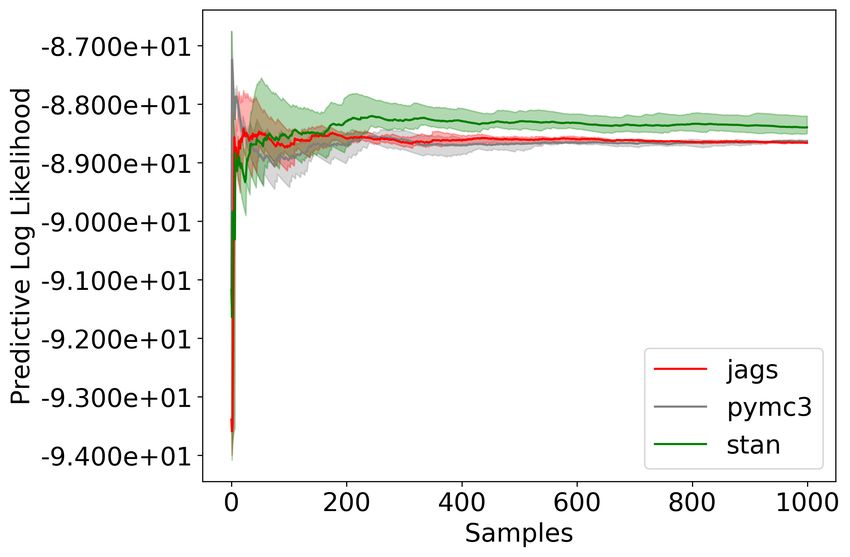
In Figure 3b, we include warmup samples in the plot. By doing so, we can also gain insights
into how quickly an algorithm adapts. We can see that Bean Machine adapts quicker than Stan.
Moreover, depending on the use-case, some metrics might be more informative to the end-users
than others. For example, we can see from Table 2 that Stan is faster than BeanMachine, but
BeanMachine generates more independent samples per time as nef f /s is higher.
5 NOISY-OR TOPIC MODEL
Inferring topics from the words in a document is a crucial task in many natural language processing
tasks. The noisy-or topic model [Liu et al. 2016] is one such example. It is a Bayesian network
consisting of two types of nodes; one type are the domain key-phrases (topics) that are latent while
others are the content units (words) which are observed. Words have only topics as their parents.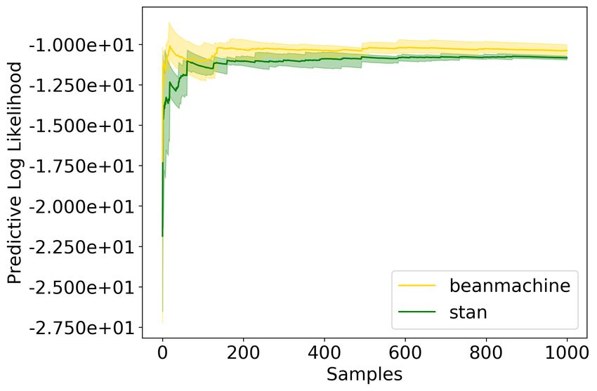
PPL Bench: Evaluation Framework For Probabilistic Programming Languages                                             5

                 (a) N = 20K, K = 10                     (b) N = 200K, K = 10 (warm up samples included)

                  Fig. 3. Predictive log likelihood against samples for Robust Regression

To capture hierarchical nature of topics, they can have other topics as parents. For model definition,
see Appendix 8.3.
   For the experiment, we first sample the model structure. This consists of determining the children
of each node in the graph, and the corresponding weight associated with the edge. Next, the key-
phrase nodes are sampled once; and two instances of content units are sampled keeping the
key-phrase nodes fixed. One instance is passed to PPL implementation for inference, while the
other is used to compute posterior predictive of the obtained samples.

5.1   Stan Implementation
The model requires support for discrete latent variables, which Stan does not have. As a workaround,
we did a reparameterization; the discrete latent variables with values "True" and "False" which denote
whether a node is activated or not are instead represented as 1-hot encoded vectors[Maddison et al.
2016]. Each element of the encoded vector is now a real number substituting a boolean variable.
"True" is represented by [1, 0] and "False" by [0, 1] in the 1-hot encoding; a relaxed representation of
a true value, for example, might look like [0.9999, 0.0001]. The detailed reparameterization process
is as follows: We encode the probabilities of a node in a parameter vector α = [α true, α false ], then
choose a temperature parameter τ = 0.1. For each key-phrase, we assign an intermediate random
variable X j :

                                                                                              nef f /s
                                              PPL     Words   Topics Time(s)
                                                                                     min      median      max
                                              Stan      300      30       37.58      17.50      79.83      80.39
                                              Jags      300      30         0.17   15028.96   17350.35   18032.36
                                             PyMC3      300      30        38.05    39.50      78.83      79.33
                                              Stan     3000     100       438.74     2.27       6.84       7.00
                                              Jags     3000     100         0.68   3773.66    4403.28    4504.26
                                             PyMC3     3000     100       298.79     3.96      10.04      14.72
                                                Table 3. Runtime and nef f /s for Noisy-Or Topic Model.

   From Figure 4, we can see that all PPLs converge to the same predictive log likelihood. We see that
JAGS is extremely fast at this problem because it is written in C++ while PyMC3 is Python-based.
We suspect that Stan is slower then PyMC3 and JAGS because of the reparameterization which
introduces twice as many variables per node.
Sourabh Kulkarni, Kinjal Divesh Shah, Nimar Arora, Xiaoyan Wang, Yucen Lily Li, Nazanin Khosravani Tehrani, Michael
6 Tingley, David Noursi, Narjes Torabi, Sepehr Akhavan Masouleh, Eric Lippert, and Erik Meijer
(a) 30 Topics, 300 Words (b) 100 Topics, 3000 Words
Fig. 4. Predictive log likelihood against samples for Noisy-Or Topic Model
6 CROWDSOURCED ANNOTATION MODEL
There exist several applications where the complexity and volume of the task requires crowdsourcing
to a large set of human labelers. Inferring the true label of an item from the labels assigned by
several labelers is facilitated by this crowdsourced annotation model[Passonneau and Carpenter
2014]. The model takes into consideration an unknown prevalence of label categories, an unknown
per-item category, and an unknown confusion matrix per-labeler. For model definition, see 8.4
6.1 Results
nef f /s
PPL Time(s)
min median max
Stan-MCMC 484.59 2.14 4.22 10.45
Stan-VI (meanfield) 15.23 0.48 7.86 216.35
Stan-VI (fullrank) 35.79 0.12 0.20 84.16
Table 4. Runtime and nef f /s for Crowd
Sourced Annotation Model with items=10K and
Fig. 5. Predictive log likelihood against samples labelers=100
for Crowd Sourced Annotation Model
PPL Bench can also benchmark different inference techniques within a PPL. Here, we benchmark
Stan’s NUTS against Stan’s VI methods, using both meanfield as well as fullrank algorithm. We
notice that VI using meanfield algorithm is indistinguishable from NUTS. However, VI using
fullrank converges to a slightly different predictive log likelihood.
7 CONCLUSION
We have provided a modular benchmarking framework for evaluating PPLs. In its current form,
this is a very minimal benchmarking suite, but we hope that it will become more diverse with
community contributions. Our work to standardize the evaluation of inference should aid scientific
development in this field, and our focus on popular statistical models should encourage overall
industrial deployments of PPLs.PPL Bench: Evaluation Framework For Probabilistic Programming Languages 7
REFERENCES
Nimar S. Arora, Nazanin Khosravani Tehrani, Kinjal Divesh Shah, Michael Tingley, Yucen Lily Li, Narjes Torabi, David
Noursi, Sepehr Akhavan Masouleh, Eric Lippert, and Erik Meijer. 2019. Newtonian Monte Carlo: a second-order gradient
method for speeding up MCMC. In Association for Advancement in Approximate Bayesian Inference (AABI).
Steve Brooks, Andrew Gelman, Galin Jones, and Xiao-Li Meng. 2011. Handbook of Markov Chain Monte Carlo. CRC press.
Bob Carpenter, Andrew Gelman, Matthew D Hoffman, Daniel Lee, Ben Goodrich, Michael Betancourt, Marcus Brubaker,
Jiqiang Guo, Peter Li, and Allen Riddell. 2017. Stan: A probabilistic programming language. Journal of statistical software
76, 1 (2017).
Marco Cusumano-Towner and Vikash K Mansinghka. 2018. A design proposal for Gen: probabilistic programming with
fast custom inference via code generation. In Proceedings of the 2nd ACM SIGPLAN International Workshop on Machine
Learning and Programming Languages. ACM, 52–57.
Hong Ge, Kai Xu, and Zoubin Ghahramani. 2018. Turing: A language for flexible probabilistic inference. In International
Conference on Artificial Intelligence and Statistics. 1682–1690.
Andrew Gelman, John B Carlin, Hal S Stern, David B Dunson, Aki Vehtari, and Donald B Rubin. 2013. Bayesian data analysis.
Chapman and Hall/CRC.
Zoubin Ghahramani. 2015. Probabilistic Machine Learning and Artificial Intelligence. Nature 521, 7553 (2015), 452.
Peter W Glynn and Donald L Iglehart. 1989. Importance sampling for stochastic simulations. Management Science 35, 11
(1989), 1367–1392.
Noah Goodman, Vikash Mansinghka, Daniel M Roy, Keith Bonawitz, and Joshua Tenenbaum. 2008. Church: a language for
generative models with non-parametric memoization and approximate inference. In Uncertainty in Artificial Intelligence.
Alp Kucukelbir, Dustin Tran, Rajesh Ranganath, Andrew Gelman, and David M Blei. 2017. Automatic differentiation
Variational Inference. The Journal of Machine Learning Research 18, 1 (2017), 430–474.
Jialu Liu, Xiang Ren, Jingbo Shang, Taylor Cassidy, Clare R Voss, and Jiawei Han. 2016. Representing Documents via Latent
Keyphrase Inference. In Proceedings of the 25th international conference on World Wide Web. International World Wide
Web Conferences Steering Committee, 1057–1067.
Chris J Maddison, Andriy Mnih, and Yee Whye Teh. 2016. The concrete distribution: A continuous relaxation of discrete
random variables. arXiv preprint arXiv:1611.00712 (2016).
Vikash Mansinghka, Daniel Selsam, and Yura Perov. 2014. Venture: a higher-order probabilistic programming platform with
programmable inference. arXiv preprint arXiv:1404.0099 (2014).
Brian Milch, Bhaskara Marthi, Stuart Russell, David Sontag, Daniel L. Ong, and Andrey Kolobov. 2005. BLOG: Probabilistic
models with unknown objects. In IJCAI International Joint Conference on Artificial Intelligence. 1352–1359.
Rebecca J Passonneau and Bob Carpenter. 2014. The benefits of a model of annotation. Transactions of the Association for
Computational Linguistics 2 (2014), 311–326.
Avi Pfeffer. 2001. IBAL: A probabilistic rational programming language. In IJCAI. Citeseer, 733–740.
Martyn Plummer et al. 2003. JAGS: A program for analysis of Bayesian graphical models using Gibbs sampling. In Proceedings
of the 3rd international workshop on distributed statistical computing, Vol. 124. Vienna, Austria., 10.
Peter J Rousseeuw and Annick M Leroy. 2005. Robust regression and outlier detection. Vol. 589. John wiley & sons.
John Salvatier, Thomas V. Wiecki, and Christopher Fonnesbeck. 2016. Probabilistic programming in Python using PyMC3.
PeerJ Computer Science 2 (apr 2016), e55. https://doi.org/10.7717/peerj-cs.55
David Spiegelhalter, Andrew Thomas, Nicky Best, and Wally Gilks. 1996. BUGS 0.5: Bayesian inference using Gibbs sampling
manual (version ii). MRC Biostatistics Unit, Institute of Public Health, Cambridge, UK (1996), 1–59.
Python Core Team. 2019. Python: A dynamic, open source programming language. Python Software Foundation. https:
//www.python.org/
Nazanin Tehrani, Nimar S. Arora, Yucen Lily Li, Kinjal Divesh Shah, David Noursi, Michael Tingley, Narjes Torabi, Sepehr
Masouleh, Eric Lippert, and Erik Meijer. 2020. Bean Machine: A Declarative Probabilistic Programming Language For
Efficient Programmable Inference. In Probabilistic Graphical Models (PGM).
Noel van Erp and P.H.A.J.M. Gelder. 2013. Bayesian logistic regression analysis. (08 2013), 147–154. https://doi.org/10.
1063/1.4819994
Martin J Wainwright, Michael I Jordan, et al. 2008. Graphical models, exponential families, and variational inference.
Foundations and Trends® in Machine Learning 1, 1–2 (2008), 1–305.Sourabh Kulkarni, Kinjal Divesh Shah, Nimar Arora, Xiaoyan Wang, Yucen Lily Li, Nazanin Khosravani Tehrani, Michael
8 Tingley, David Noursi, Narjes Torabi, Sepehr Akhavan Masouleh, Eric Lippert, and Erik Meijer
8 APPENDIX A - STATISTICAL MODEL DEFINITIONS
8.1 Bayesian Logistic Regression
α ∼ Normal(0, 10, size = 1),
β ∼ Normal(0, 2.5, size = K),
X i ∼ Normal(0, 10, size = K) ∀i ∈ 1 . . . N
µi = α + Xi T β ∀i ∈ 1..N
Yi ∼ Bernoulli(logit = µ i ) ∀i ∈ 1..N .
8.2 Robust Regression
ν ∼ Gamma(2, 10)
σ ∼ Exponential(1.0)
α ∼ Normal(0, 10)
β ∼ Normal(0, 2.5, size = K)
X i ∼ Normal(0, 10, size = K) ∀i ∈ 1 . . . N
µi = α + β T Xi ∀i ∈ 1 . . . N
Yi ∼ Student-T(ν, µ i , σ ) ∀i ∈ 1 . . . N
8.3 Noisy-OR Topic Model
Let Z be the the set of all nodes in the network. Each model has a leak node O which is the parent
of all other nodes. The set of keyphrases is denoted by K and the set of content units is represented
as T .
|Children(Ki )| ∼ Poisson(λ = 3) ∀i ∈ 1 . . . K
Woj ∼ Exponential(0.1) ∀j ∈ 1 . . . Z
Wi j ∼ Exponential(1.0) ∀i, j where i ∈ Parents(Z j )
Õ
P(Z j = 1|Parents(Z j )) = 1 − exp(−Woj − (Wi j ∗ Z i ))
i
Zj ∼ Bernoulli(P(Z j = 1|Parents(Z j )))
8.4 Crowd Sourced Annotation Model
There are N items, K labelers, and each item could be one of C categories. Each item i is labeled by
a set Ji of labelers. Such that the size of Ji is sampled randomly, and each labeler in Ji is drawn
uniformly without replacement from the set of all labelers. zi is the true label for item i and yi j is
the label provided to item i by labeler j. Each labeler l has a confusion matrix θl such that θlmn isPPL Bench: Evaluation Framework For Probabilistic Programming Languages 9
the probability that an item with true class m is labeled n by l.
1 1
π ∼ Dirichlet , . . . ,
C C
zi ∼ Categorical(π ) ∀i ∈ 1 . . . N
θlm ∼ Dirichlet(αm ) ∀l ∈ 1 . . . K, m ∈ 1 . . . C
|Ji | ∼ Poisson(Jloc )
l ∈ Ji ∼ Uniform(1 . . . K) without replacement
yil ∼ Categorical(θl zi ) ∀l ∈ Ji
Here αm ∈ R+C . We set αmn = γ · ρ if m = n and αmn = γ · (1 − ρ) · C−1 1
if m , n. Where γ is the
concentration and ρ is the a-priori correctness of the labelers. In this model, Yil and Ji are observed.
In our experiments, we fixed C = 3, Jloc = 2.5, γ = 10, and ρ = 0.5.You can also read