Atmospheric composition coupled model developments and surface flux estimation - Saroja Polavarapu - ECMWF
←
→
Page content transcription
If your browser does not render page correctly, please read the page content below
Atmospheric composition coupled
model developments and surface
flux estimation
                  Saroja Polavarapu

           Climate Research Division, CCMR
        Environment and Climate Change Canada

  ECMWF seminar: Earth System Assimilation, 12 Sept. 2018
OUTLINE
1. The carbon cycle: a coupled data assimilation problem
2. Meteorology/constituent coupling in models
       ▪ Sources of coupling in online constituent transport models
       ▪ Impacts of constituents on meteorological forecasts
3. Data assimilation for constituents and surface fluxes
       ▪   Inverse modelling with a Chemistry Transport Model (CTM)
       ▪   Constituent transport model error
       ▪   Impact of meteorological uncertainty on constituent forecasts
       ▪   Coupled meteorological, constituent state, flux estimation
4. Challenges of greenhouse gas surface flux (emissions)
   estimation

                             Page 2 – September 12, 2018
1. The carbon cycle: a
coupled data assimilation
         problem

         Page 3 – September 12, 2018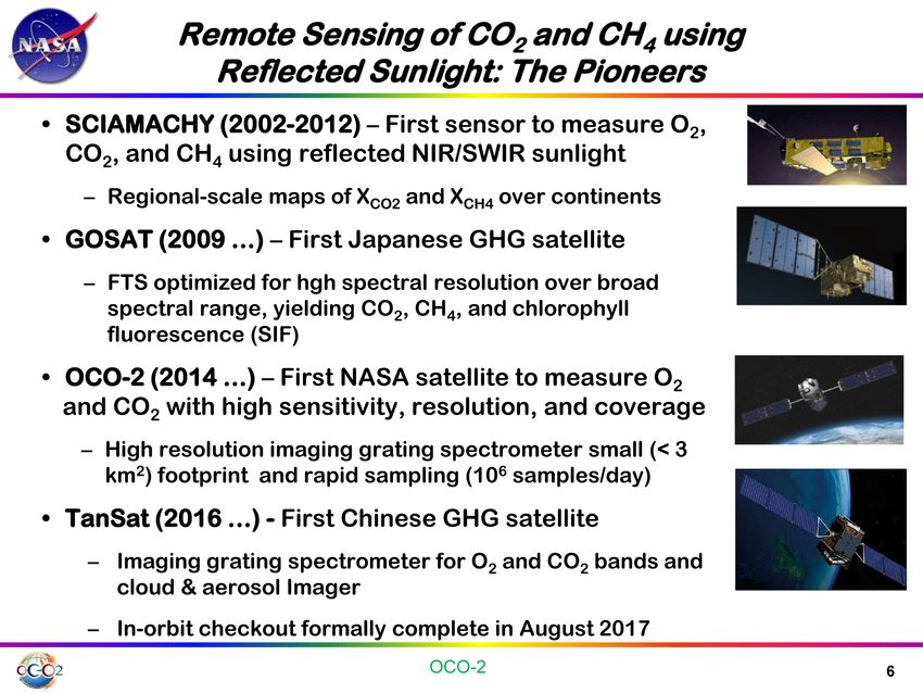
The Global Carbon Cycle
                                    http://www.scidacreview.org/0703/html/biopilot.html

                                                              1 Pg = 1 Gt = 1015 g
                                                Pg C/yr
                                                                Net surface to
                                                                atmosphere flux for
                                                                biosphere or ocean is
                                                                a small difference
                                                                between two very
                                                                large numbers
            Earth’s crust 100,000

• The natural carbon cycle involves CO2 exchange between the
  terrestrial biosphere, oceans/lakes and the atmosphere.
• Fossil fuel combustion and anthropogenic land use are additional
  sources of CO2 to the atmosphere.
                            Page 4 – September 12, 2018
Net perturbations to global carbon
budget                  LeQuéré et al. (2018, ESSDD)

                                    • Based on 2005-2014
                                    • 44% of emissions remain
                                        in atmosphere
                                    •   28% is taken up by
                                        terrestrial biosphere
                                    •   22% is taken up by
                                        oceans

                                                 1 Pg = 1 Gt = 1015 g

                   Page 5 – September 12, 2018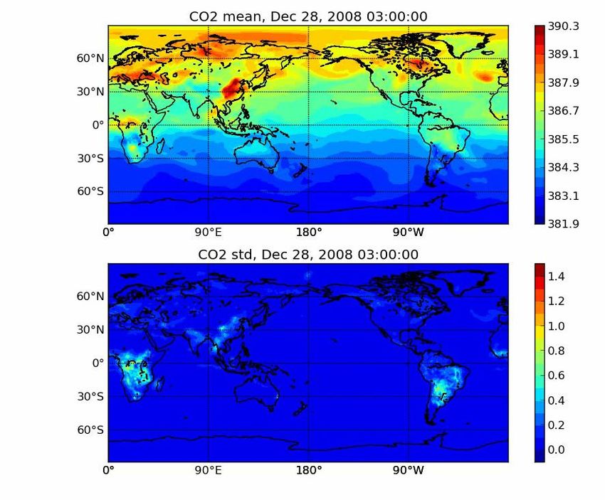
Interannual variability
                                                             IPCC AR5 WG1 2013

                                                          We need to better
                                                          understand biospheric
                                                          sources and sinks

The largest uncertainty and interannual variability in the global CO2
uptake is mainly attributed to the terrestrial biosphere
                            Page 6 – September 12, 2018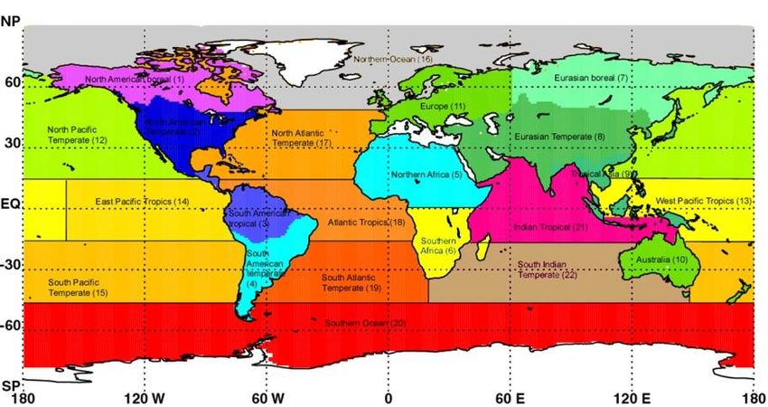
Interannual variability in
atmospheric CO2 due to climate
                                                                 Keeling et al. (2005)

               *       *                         *        *El Niño
                                                           Pinotubo

                                                          75% of interannual
                                                          variability in CO2 growth
                                                          rate is related to ENSO
                                                          and volcanic activity
                                                          (Raupach et al. 2008)

• Tropical CO2 flux goes from uptake to release in dry, warm ENSO.
• More CO2 uptake by plants with more diffuse sunlight and cooler
  temperatures after volcanic eruptions.
                            Page 7 – September 12, 2018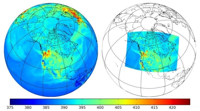
Coupled Carbon Data Assimilation
Systems

  http://www.globalcarbonproject.org/misc/JournalSummaryGEO.htm

                         Page 8 – September 12, 2018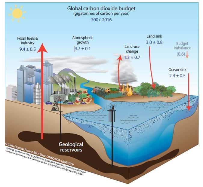
Coupled land/ocean/atmosphere
                                https://www.esrl.noaa.gov/gmd/ccgg/basics.html

                                          weather

http://web.mit.edu/globalchange/www/tem.html

                                Page 9 – September 12, 2018

                     https://gmao.gsfc.nasa.gov/reanalysis/MERRA-NOBM/model_description.php
CO2 Time scales
                                                               Video by Mike Neish (ECCC)
Simulation of CO2 with GEM-MACH-GHG using NOAA CarbonTracker optimized fluxes

                                                                               Colour
                                                                               bar
                                                                               range is
                                                                               3.5% of
                                                                               mean

            • Diurnal, synoptic, seasonal, annual
            • Hemispheric gradient
            • Signals are mixed by middle of Pacific ocean
                                Page 10 – September 12, 2018
Atmospheric CO2 observations
Keeling et al. (2005)
Time signals:
• Linear trend
• Seasonal cycle
• Amplitude ↓ with latitude
Page 11 – September 12, 2018Evolution of the in situ obs network
Bruhwiler et al. (2011)
29 sites 48 sites
Routine flask samples
Continuous obs
Not used flask obs
Aircraft sampling
• Original goal: Long
term monitoring of
103 sites 120 sites background sites
• Later on: Add
continental sites to
better constrain
terrestrial biospheric
fluxes at continental
scales
Page 12 – September 12, 2018Increasing in situ measurements
https://www.icos-ri.eu/greenhouse-gases
2018 ECCC GHG network
Hourly obs of CO2, CH4, CO
ICOS network has stations in 12
countries: atmospheric (30+),
Page 13 – September 12, 2018
Figure courtesy of Elton Chan (ECCC) ecosystem flux (50+) , ocean
measurements (10+)Slide from Dave Crisp, JPL
7
Page 14 – September 12, 2018WMO/UNEP - Integrated Global Greenhouse
Gas Information System (IG3IS)
https://public.wmo.int/en/resources/bulletin/integrated-global-greenhouse-gas-information-system-ig3is
Objective: Provide timely actionable GHG information to stakeholders
1. Support of Global Stocktake and national GHG emission inventories
• Establish good practices and quality metrics for inverse methods and how to
compare results to inventories
• Reconcile atmospheric measurements and model analyses (inverse modelling)
with bottom up inventories
2. Detection and quantification of fugitive methane emissions
▪ Extend methods used by EDF, NOAA and others to identify super emitters in
N.American oil and gas supply chain to countries and other sectors: offshore
platforms, agriculture, waste sector
3. Estimation and attribution of subnational GHG emissions
▪ Urban GHG information system using atmospheric monitoring, data mining and
(inverse) models, Provide sector-specific information to stakeholders
Page 15 – September 12, 2018ECMWF and CO2 monitoring
https://www.che-project.eu/
Slide from Gianpaolo Balsamo presentation at CHE workshop Feb. 2018
Page 16 – September 12, 2018The carbon cycle data assimilation
problem
• Estimating surface fluxes (emissions):
– By following the movement of carbon.
– Ultimately, we want to be able to attribute distributions to source
sectors (e.g. fossil fuel, natural, etc.)
• Multiple spheres are coupled:
– atmosphere, ocean, constituents, terrestrial biosphere
– Assimilation window lengths vary from hours to years
• Multiple time scales:
– interannual, seasonal, synoptic, diurnal
• Multiple spatial scales:
– global, regional, urban
• Long lifetime species: CO2 (~5-200 years), CH4 (~12 years)
Page 17 – September 12, 20182. Meteorology and
constituent coupling in
atmospheric models
Page 18 – September 12, 2018Coupled meteorology and chemistry
• Meteorological model equations (momentum,
thermodynamic, equation of state) mass
species
• Species continuity equation for mixing ratio:
moist air
emission, dry
deposition, wet
deposition,
Density moist air Diffusion coefficient photochemistry,
gas/particle
partitioning, etc.
• For greenhouse gases: tracer mass conservation desired
• Tracer variable: dry air mixing ratio is desired
Page 19 – September 12, 2018Lack of global dry air conservation
Takacs et al. (2015)
Global monthly mean mass anomalies
Dry air mass is not
conserved because:
1) Model conserves
moist air mass
2) Model continuity eq
does not account for
sources
3) Analysis increments
of surface P and
water vapour are not
consistent
Page 20 – September 12, 201821
Conserving tracer mass in GEM
One time step
3
Met. Dyn. Tracer adv mass fixer Physics Met. Dyn.
Psadj-dry Ps_source
1 2 Chemistry 4
5
Emission
1. The model loses mass during the dynamics step, so psadj-dry adjusts the global dry
air mass so it is conserved. The tracer mixing ratio is not adjusted even though the
dry air mass is not locally conserved.
2. Tracer mass is changed during advection so the mass fixer is applied for global
conservation. This requires knowledge of the dry air mass field (Ps, q)
3. During Physics, water vapour (q) is changed so dry air is changed so tracer needs
adjusting.
4. Mass change due to change in q from physics is added to Ps.
5. Emission is added so the tracer mass changes. q and Ps are needed.
Page 21 – September 12, 2018Processes that couple meteorological
and chemistry variables
Meteorological impacts on constituents:
• Surface pressure, water vapour through dry air mass
• Wind fields through advection
• Temperature through chemical reaction rates
• Temperature through photosynthesis, respiration
• Convection schemes: transport constituents
• Boundary layer parameterizations: transport constituents
Constituent impacts on meteorology:
• Forecast model’s radiation calculation
• Assimilation of constituents could potentially impact
– Temperature analyses through improved radiance assimilation
– Wind field analyses through coupling
Page 22 – September 12, 2018 in dynamics, covariancesCO2 and radiance assimilation
Engelen and Bauer (2012)
August 2009 mean CO2 minus 377 ppm, ~210 hPa
Bias correction has less
work to do if CO2 is a 3D
field.
Impact on temperature
analyses/forecasts is
positive at 200 hPa in
tropics, neutral elsewhere
AIRS ch. 175 ~200 hPa
Constant CO2 Bias correction Aug. 2009 Variable CO2
Page 23 – September 12, 2018Impact of assimilating CO2 , CH4 on
wind fields Massart (WMO WWRP e-news Jan. 2018)
Impact of IASI CO2 and CH4
retrievals with EnKF for Jan-Feb
2010 is positive in stratospheric
southern hemisphere
Page 24 – September 12, 20183. Data assimilation:
Constituent/flux estimation
Page 25 – September 12, 2018The surface flux estimation problem
Using atmospheric observations from the present, what
was the past flux of GHG from the surface to the
atmosphere?
observations
Prior flux estimate
Time past present
Page 26 – September 12, 2018The standard inverse modeling approach
World Data Centre for Greenhouse Gases (WDCGG) 22 TransCom regions
http://gaw.kishou.go.jp/cgi-bin/wdcgg/map_search.cgi http://transcom.project.asu.edu
Weekly avg obs
Monthly scaling factors
J F M A M J J A S O N D J F M A M J J
Page 27 – September 12, 2018
One or more yearsThe standard inverse problem for
carbon flux estimation
flux Prior flux conc obs
Spatial interpolation Forecast model
• In flux inversions, if one solves for surface fluxes only, the transport
model is needed to relate the surface flux to the observation
• Can solve inverse problem with 4D-Var
• Extension for imperfect tracer initial conditions, add a term
• Assumptions
• Anthropogenic and biomass burning emissions are perfectly known
• Observations and forecast errors are unbiased
• Prior flux error covariance is known (correctly modelled)
• Model-data mismatch covariance is known (correctly modelled)
• Perfect model assumption since forecast model is used as a strong constraint
Page 28 – September 12, 2018Fixed Lag Kalman Smoother
Peters et al. (2005, JGR)
obs
0 1 2 3 4 5 6 7 8 9 10 11 12 13 14 15 16 17 18
weekly mean flux
• e.g. CarbonTracker NOAA, CT-Europe, CT-Asia
• State vector: 5-12 sets of weekly-mean fluxes
• Lag: 5-12 weeks
• Forecast step: Persistence, static prior covariances
• Perfect model: transport model in observation operator
Page 29 – September 12, 2018Transport model is not perfect
Gurney et al. (2003, Tellus)
Zonal mean annual mean CO2
Even with the same
surface fluxes,
different models give
different CO2.
Transport model
errors are an
Range of important source of
4 ppm error in surface flux
inversions (Chevallier
et al., 2014, 2010;
Houweling et al.,2010;
Law et al., 1996)
Page 30 – September 12, 2018Forecast or “Transport error”
met state 2D flux
1) Transport model
chem state
2) True evolution
Model error
Forecast error: (1) – (2) Chem error Flux error
Higher
order
terms
Meteor. state error
Constituent error
Page 31 – September 12, 2018
Flux errorSources of constituent transport
model error
• If constituent state, meteorological state and fluxes are
perfect, the constituent forecast can still be wrong due to
model error. For CO2, sources of model error are:
– Boundary layer processes (Denning et al. 1995)
– Convective parameterization (Parazoo et al. 2008)
– Synoptic scale and frontal motions (Parazoo et al. 2008)
– Mass conservation errors (Houweling et al. 2010)
– Interhemispheric transport (Law et al. 1996)
– Vertical transport in free atmosphere (Stephens et al. 2007,
Yang et al. 2007)
– Chemistry module, if present. (CO2 is a passive tracer; CH4, CO use
parameterized climate-chemistry with monthly OH)
• Comparing CO2 simulations to observations reveals
model errors due to meteorological
Page 32 – September 12, 2018 processes leading
to feedback on meteorological modelDealing with model error: variational
approach
• Use constituent observations to constrain both fluxes and
model errors, u (3D fields of mixing ratio)
Page 33 – September 12, 2018Application of weak constraint 4D-
Var to GOSAT CH4 assimilation
Stanevich et al. (2018, ACPD*)
*To be submitted
• GEOS-Chem 4° x 5°
• 3-day forcing window
Weak constraint • Forcing over whole domain
• Weak constraint solution
better matches independent
observations
Solving for fluxes only
misattributes model errors
Strong constraint
to flux increments
Page 34 – September 12, 2018Dealing with model error: Coupled
constituent and flux estimation
Flux forecast
• Flux forecast model is persistence: Fk = I
• Chinese Tan-Tracker: GEOS-Chem, 5 week lag, weekly fluxes (Tian
et al. 2014, ACP)
• Fixed interval Ens. Kalman smoother, 3-day window (Miyazaki et al.
2011, JGR)
Page 35 – September 12, 2018Errors in meteorological analyses
Liu et al. (2011, GRL)
Uncertainty in CO2 due to
errors in wind fields is
1.2–3.5 ppm at surface
and 0.8–1.8 ppm in
column mean fields.
Global annual mean of
natural fluxes is ~2.5 ppm
Using same sources/sinks, same model, same initial condition, CO2
forecasts are still different due to errors in wind fields.
Page 36 – September 12, 2018Coupled global weather and
greenhouse gas models
Initial CO2 on
1 Jan 2009 from
CarbonTracker
Sub-daily fluxes (biospheric, ocean, anthropogenic, biomass burning)
3-hourly CT2013B fluxes from NOAA CarbonTracker
Coupled systems using global models:
• ECMWF CAMS (Agusti-Panareda et al. 2014)
• NASA GMAO (Ott et al. 2015)
• ECCC (Polavarapu etPageal. 2016)
37 – September 12, 2018Experimental design: predictability
Reference cycle Climate cycle
• Analyses constrain CO2 transport using observed
meteorology even with no CO2 assimilation
• What if we don’t use analyses (after the initial time) and
replace them with 24h forecasts? Climate cycle
• Climate cycle will drift from control cycle which uses
analyses
Page 38 – September 12, 2018Predictability error definition used
• Drift of climate cycle from reference cycle:
• E=(CO2clim-CO2ref)
• A measure of variability:
• P = Global mean (zonal standard deviation (E))
• Normalize by variability in full state itself (at initial time):
• P0 = Global mean (zonal standard deviation (CO2ref(t0)))
• Define Normalized Predictability error:
• N=P/P0
• Dimensionless
• Can compare different variables, (e.g. T, vorticity, divergence)
• NNormalized predictability error for Jan 2009
Page 40 – September 12, 2018Climate time scales: seasonal
• CO2 predictability is short ~2 days in the free troposphere
and follows pattern of wind field predictability. CO2
predictability increases near the surface and in the lower
stratosphere
• Can we see predictability on longer (sub-seasonal to
seasonal) time scales?
• Do a spherical harmonic decomposition of drift E and
average over one month of spectra, and over 12 model
levels
Page 41 – September 12, 2018July 2009
Largest scales are
predictable in July
Predictability error
Where does this
CO2 state predictability come from?
• CO2 surface fluxes
• Land/ocean surface
Page 42 – September 12, 2018Experimental design: analysis error
Reference cycle Perturbed analysis cycle
• Meteorological analyses keep our CO2 transported by
realistic wind fields. But analyses are not perfect. What
is the impact of analysis error on CO2 spatial scales?
• Experiment: Perturb reference analyses by error
• Analysis error proxy: Cycle with analysis 6h early
Page 43 – September 12, 2018Impact of meteorological analysis uncertainty
Polavarapu et al. (2016, ACP)
Imperfect winds
No wind info
CO2 state ref
2000 500
400 km 770 km 1000 km 1000 km
• Error spectra asymptote to predictability error spectra. For smaller
spatial scales, we don’t gain much over predictability error.
• For some wavenumber, the power in this error equals that in the
state itself (red arrows). There is a spatial scale below which CO2
is not resolved due to meteorological analysis uncertainty. This
spatial scale increases with altitude.
Page 44 – September 12, 2018Spatial scales seen in fluxes
If CO2 can be reliably simulated only for large spatial scales, this
translates to flux uncertainties which are unaccounted for.
observations
Prior flux estimate
Time past present
Page 45 – September 12, 2018Implications on flux inversions
If CO2 can be reliably simulated only for large spatial scales, this
translates to flux uncertainties which are unaccounted for.
observations
Posterior flux estimate
Time past present
Page 46 – September 12, 2018Implications on flux inversions
If CO2 can be reliably simulated only for large spatial scales, this
translates to flux uncertainties which are unaccounted for.
observations
Posterior flux estimate
Time past present
Page 47 – September 12, 2018Coupled meteorology, constituent
and flux estimation
• Assimilate meteorology and chemistry observations
• State vector (x, c, s): meteorology, chemistry, fluxes
• Meteorological uncertainties (e.g. boundary layer,
convection) can be simulated with an EnKF
• Demonstrated w LETKF with a 6h window (Kalnay group)
– OSSEs w SPEEDY model: Kang et al. (2011, JGR; 2012, JGR)
• Flux estimates obtained through cross covariances with
CO2 state estimates through ensemble requires a good
state estimate constrained by lots of observations
• How to deal with differing assimilation window lengths:
6h – meteorology, CO2 state, weeks/months for fluxes?
Page 48 – September 12, 2018Challenges of GHG data assimilation
• Multiple time scales: diurnal, synoptic, seasonal, interannual
• Multiple spatial scales: Global, regional, urban
• Multiple systems: Atmosphere, ocean, constituents, biosphere. How
to deal with different assimilation window lengths?
• Multiple chemical species may be needed to attribute components of
fluxes to natural or anthropogenic origin
• New satellite observations: need to improve bias corrections,
develop inter-satellite bias corrections
• Need independent obs for validation, anchoring bias corrections
• Moving to near-real-time systems
Page 49 – September 12, 2018EXTRA SLIDES
Page 50 – September 12, 2018Spatial scales of fluxes seen in CO2
Polavarapu et al. (2018, ACP)
Zonal standard deviation of DCO2 (global mean)
Compare:
GOSAT GEOS-Chem/GEM
In situ GEOS-Chem/GEM
CO2 (fluxprior, metref) – CO2 (fluxpost,metref)
and
CO2 (fluxpost, metref) – CO2 (fluxpost,metpert)
Posterior fluxes from GOSAT assimilation
Posterior fluxes from flask obs assimilation
• Impact of updated fluxes on CO2 exceeds CO2 uncertainty due to
meteorological uncertainty most seasons, if GOSAT data is used
• This occurs only in boreal summer, if flask data is used
Page 51 – September 12, 2018CO2 state
Pred. error
Page 52 – September 12, 2018
Land and ocean surface affects CO2 predictabilityThe flux estimation problem
Using atmospheric observations from the present, what
was the past flux of GHG from the surface to the
atmosphere?
observations
CO2 forecast Fluxes
Forecast model Model error
Meteorological CO2 analysis
analysis
Prior flux estimate
Time past present
Page 53 – September 12, 2018Dealing with model error: Coupled
state/flux estimation Miyazaki (2011, JGR)
• Fixed interval Kalman
smoother
• 3-day window
• 48 members
• Flux forecast: persistence
• Temporal and spatial localization is done.
• CO2 mass not conserved due to analysis increments
Page 54 – September 12, 2018Coupled state/flux estimation
Tian et al. (2014, ACP)
• EnVar, GEOS-Chem
• State vector: CO2, l
• Flux forecast:
persistence
• Temporal and spatial localization is done.
• CO2 mass not conserved due to analysis increments
Page 55 – September 12, 2018Predictability of CO2 in a regional model
Jinwoong Kim (ECCC)
Reference cycle (GLBref) 90 km 10 km
Climate IC (GLBclim)
Reg. IC LBC
LAM ref-ref Analysis GLBref
LAM clim-ref Forecast GLBref
LAM ref-clim Analysis GLBclim
LAM clim-clim Forecast GLBclim
Perturbed cycle (GLB pert)
LAM pert-ref Perturbed GLBref
Analysis
LAM ref-pert Analysis GLBpert
Page 56 – September 12, 2018
LAM pert-pert Perturbed GLBpert
AnalysisPredictability of CO2 in a regional model
Jinwoong Kim (ECCC)
June 2015 monthly mean spectra
Wrong BC
Wrong IC
L01-12 lower troposphere L13-24 mid troposphere
Page 57 – September 12, 2018
L25-36 upper troposphere L37-48 stratosphereOptimal window length for CO2 flux
Liu et al. (2018, GMDD)
With an assimilation window of 1 day, the optimal observation window is 8
days based on OSSEs with GEOS-Chem and OCO-2 data. LETKF with
GEOS-Chem coupled CO2 state and flux estimation was used.
Page 58 – September 12, 2018Evolution of ensemble spread
Animation of column mean CO2
Dec. 28, 2008 to Jan. 23, 2009
Ensemble
mean
Ensemble
spread
Page 59 – September 12, 2018How does uncertainty in winds affect
CO2 spread?
2009012206 2009012206
CO2 ens std dev at eta=0.997 ppmv U ens std dev at eta=0.994 ECLA RMS 2009012200 ±2 days mg/m2/s
m/s
• CO2 spread (left) does not mainly resemble spread in
winds (middle) but rather the spatial variability of
biospheric fluxes (right)
• Only where tracer gradients exists does uncertainty in
winds matter Page 60 – September 12, 2018Ensemble Kalman Filter – first look
• No tracer assimilation, only passive advection
• Testing with 64 ensemble members, 0.9° grid spacing
• Start on 28 Dec 2008. Run for 4 weeks to 23 Jan 2009
• All members have same initial CO2 and same fluxes.
Spread is due to spread in winds only.
• Winds differ among ensemble members due to
differences in: model parameters (convection scheme,
parameters involved in PBL model, diffusion of potential
temperature, etc. ), observation error perturbations
• How does uncertainty in winds affect CO2 spread?
Page 61 – September 12, 2018Slide from Dave
Crisp, JPL
Page 62 – September 12, 2018Slide from Dave
Crisp, JPL
Page 63 – September 12, 2018Slide from Dave Crisp, JPL Page 64 – September 12, 2018
CO2 Variations with height
            Park Falls: 29 May-10 June, 1996            Olsen and Randerson (2004, JGR)

                  Column CO2                         • Diurnal variations, linked to
                                                          surface sources and sinks, are
                                                          strongly attenuated in the free
                                                          troposphere
                                                     • Diurnal variations in column CO2
                                                          are less than 1 ppm
                                                     • Large changes in the column
                                                          reflect the accumulated influence
                                                          of the surface sources and sinks
                                                          on timescales of several days
                Surface CO2

Diurnally
varying
                                                           5-day running
surface
                                                           mean surface
fluxes
                                    Page 65 – September 12,fluxes
                                                            2018
Inversions using surface network
Peylin et al. (2013)
• Inversion methods
differ in:
– Methodology
– Observations
▪ Sfc: 100 flask +
continuous
– A priori fluxes
– Transport models
• Interannual variability
is similar and due to
1 5-6
2 7-8
land
39
4 10
Page 66 –11
September 12, 2018Spatial information
Peylin et al. (2013)
• Good agreement on
global fluxes and
partition into land and
ocean
Not as good agreement
on spatial distributions 25N-25S
even for very large
regions (only 3 latitude
bands)
Page 67 – September 12, 2018Flux inversions using GOSAT data
Houweling et al. (2015, ACP)
Page 68 – September 12, 2018You can also read