Would you jump? or the uncertainty of living R. Muñoz-Carpena, Ph.D., Professor Agricultural & Biological Engineering
←
→
Page content transcription
If your browser does not render page correctly, please read the page content below

Would you jump?
or the uncertainty of living…
R. Muñoz-Carpena, Ph.D., Professor
Agricultural & Biological Engineering

 Based on A. Saltelli (2004) Sensitivity Analysis in
 Practice. Wiley: London Agricultural and Biological Engineering
Agricultural and Biological Engineering
Would you jump?
 Class discussion (1)…

 Agricultural and Biological Engineering

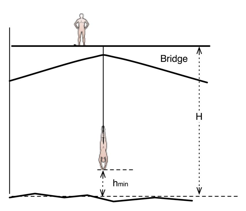
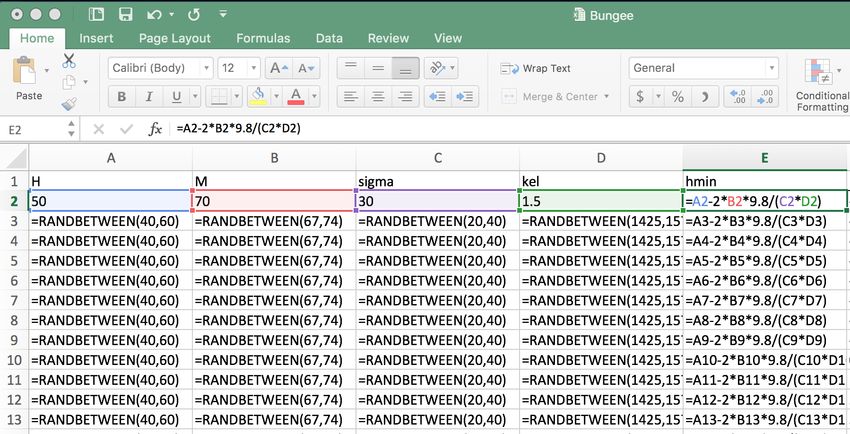
Bungee Jumping Model
 Simplified solution to linear oscillator
M
 equation (string length=0):

 2Mg
 hmin =H−
 σ, kel
 kelσ
 hmin= minimum distance to surface [m]
 H=distance from platform to surface[m]
 M=mass of jumper [kg]
 σ= number of strands in cord [-]
 Floor kel=elastic constant of material [N/m]≈1.5
 g= gravity constant (9.81 m/s2)

 Agricultural and Biological Engineering

σ

Agricultural and Biological Engineering

Bungee Jumping Model
Example: a 70 Kg (M) person jumping 50 m (H) with a cord made of
30 strands (σ=30 ) and elasticity kel = 1.5 N/m
à hmin = ? (Let’s calculate in Excel!!)

 2Mg
 hmin =H− = 19.5 m = 62 ft
 kelσ
 Agricultural and Biological Engineering
And now…
Would you jump?
Class discussion redux (2) …

 Agricultural and Biological Engineering
On the uncertainty of life…
 Monte-Carlo Uncertainty Analysis
 Uncertain input factors* when jumping?

 • H: U(40,60) (m, bottom variation, topo survey)
 • M: U(67,74) (kg, ±5%, physiological)
 • σ: U(20,40) ([-], based on vendor survey)
 • kel: U(1.475-1.525) (N/m, 5% manufacturer)

 2Mg
 hmin =H−
 kelσ
(*) Input factors: anything that would change the model/system
outputs (parameters, initial and boundary conditions)
 Agricultural and Biological Engineering
Let’s calculate probable values for each factor and
propagate those into the hmin model –> Monte Carlo UA

… x 3000 times 2Mg
 hmin =H−
 kelσ Agricultural and Biological Engineering
Monte-Carlo Uncertainty Analysis (UA)
 H: U(40,60) (m, bottom variation, survey)
 M: U(67,74) (kg, ±5%, physiological)
 σ: U(20,40) (no. based on vendor survey)
 kel:U(1.475-1.525) (5% manufacturer)

 … Negative value =

 ✟!!
 … x 3000 times
 Agricultural and Biological Engineering
Monte-Carlo Uncertainty Analysis (UA)
 Probable values of hmin
 120 120.00%

 100 100.00%

 80 80.00%
Frequency

 60 60.00%

 40 40.00%

 20 20.00%

 0 0.00%
 p(hmin
And now…
Would you jump?
Class discussion redux (3)…

 Agricultural and Biological Engineering
Why so much uncertainty?
• What are the important factors controlling it?
• Can we reduce/control uncertainty through
 management/policy actions?
• Can we control/reduce uncertainty in complex
 environmental systems, with many inputs
 where the response is more that the sum of
 the individual components (interactions)?

 Agricultural and Biological Engineering
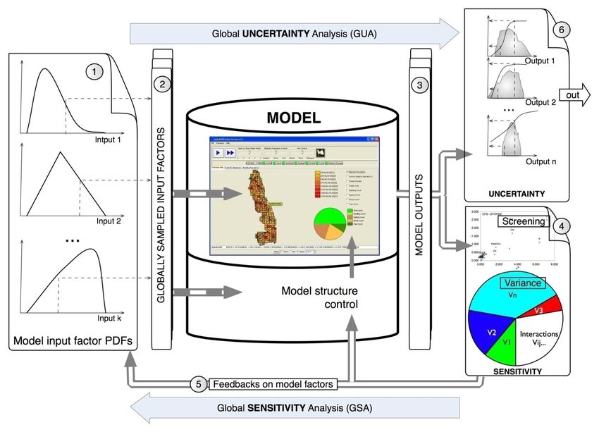
Global Sensitivity & Uncertainty Analysis (GSUA)
 Some definitions:
 • Mathematical models are built in the presence of
 uncertainties of various types (input variability,
 model algorithms, model calibration data, and
 scale).
 • Uncertainty analysis is used to propagate all these
 uncertainties, using the model, onto the model
 output of interest
 • Sensitivity analysis is used to determine the
 strength of the relation between a given uncertain
 input and the output

 Agricultural and Biological Engineering
Global Sensitivity/Uncertainty Analysis
 A B
 WHY/WHEN? Apportions output variance into input factors
A
 C GLOBAL SENSITIVITY ANALYSIS
 C

B ? ?

 INPUT ?
 MODEL
 FACTORS OUTPUTS

 100%
 300 80%

 UNCERTAINTY ANALYSIS HOW MUCH?

 Frequency
 200 60%

 CDF
 40%
 100
 20%
 0 0%

 0.00
 0.03
 0.06
 0.09
 0.13
 0.16
 0.19
 0.22
 0.25
 0.28
 0.31
 0.34
 0.38
 Bin

 Propagates input factor variability into output
 Agricultural and Biological Engineering
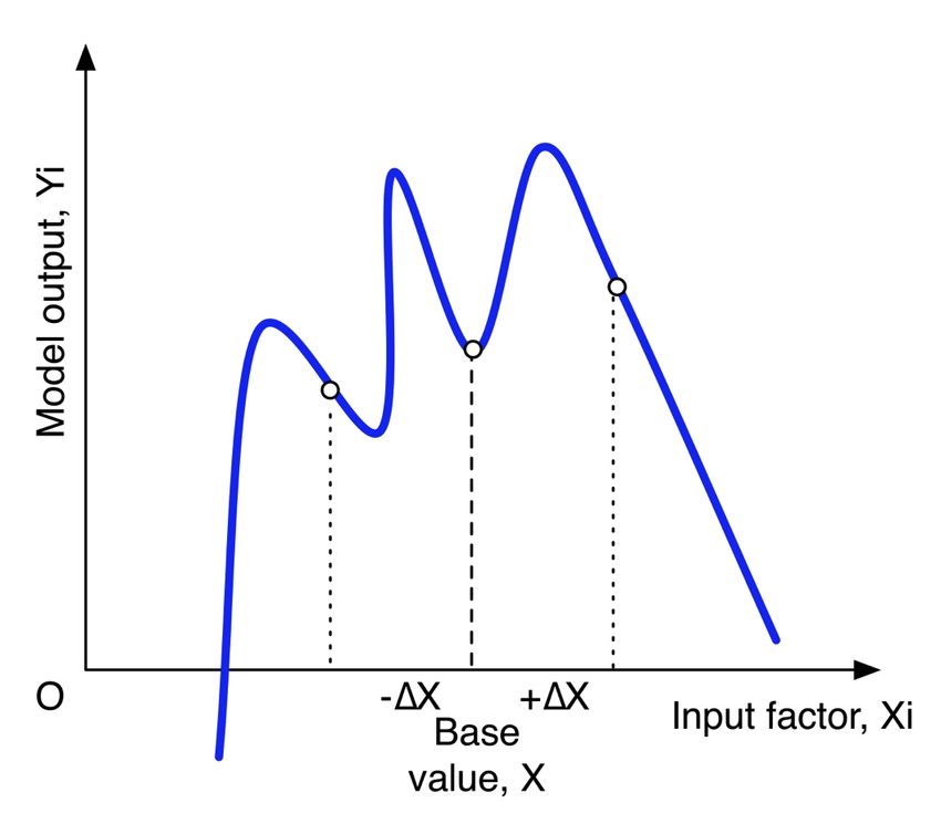
Classical SA approach - derivative local OAT
• Often model sensitivity is expressed as a simple
 derivative of model output (y) with respect to the
 variation of a single input factor (xi):
 – S = ∂y/∂xi (absolute sensitivity)
 – Sr= (xm/ym)(∂y/∂xi) (relative sensitivity w/means)
 – Ss=(sxi/sy)(∂y/∂xi)(relative sensitivity w/uncertainty)
• While the last two measures are unit independent,
 sy requires an uncertainty analysis of the model
 output.
• These derivative measures can be efficiently
 computed (direct differentiation of model
 equations, automatic differentiation algorithms,
 etc.).
• Local, One-factor-At-a-Time (OAT).
 Agricultural and Biological Engineering
• However, these measures only provide local
 information of one-factor-at-a-time (OAT). Often the
 derivative is non-linear.

 Local abs. sens.
 Simple 2-parameter reversible
 chemical reaction. Values of local
 sensitivity indexes: (a) absolute; (b)
 bottom pseudoglobal or
 normalized by ski/ s[A]) input range

 Local relative sens.

• What happens to the more common problem of a
 model driven by more than one factor with varying
 effects across the input range?
 Agricultural and Biological Engineering
Dependency of sensitivity with time

k1 ~N(3,0.3)
k-1~N(3,1.0)

Scatter plots of [A] versus k1,k-1 at time t = 0.3 and t = 0.06. k1 appears more influential than
k-1 at t = 0.06, while the reverse is true at t = 0.3
 Agricultural and Biological Engineering
Global Sensitivity Analysis
• Local vs. global sensitivity analysis (SA)

 Local SA (classic) Global SA
Model Linear No
 Monotonic assumptions
 additive
No. of factors O-A-T All together
Factor range Local Whole PDF
 (derivative)
Interactions No Yes

 Agricultural and Biological Engineering
Global Sensitivity Analysis
 HOW MUCH, WHY, WHEN…
 • surprise the analyst,
 • find technical errors in the model,
 • gauge model adequacy and relevance,
 • identify critical regions in the space of the inputs
 (including interactions),
 • establish priorities for research,
 • simplify models,
 • verify if policy options make a difference or can be
 distinguished.
 • anticipate (prepare against) falsifications of the analysis
 • …
 Adpt. from [Saltelli, 2006, SAMO Venice]
 Agricultural and Biological Engineering
• Potentially large input set.

How to handle the model evaluation with many inputs
at the time?

• Effect of model structure complexity
 on sensitivity of inputs.
Often we can have several choices of model
formulation, each adding, removing or simply
changing the conceptual basis of existing
components. What is the effect the model output and
other inputs in the model of this changes in the model
structure?
 Agricultural and Biological Engineering
GSUA evaluation framework
For model with large number of factors a two-step
global process is recommended:

1. Qualitative Screening with limited number of simulation (p.ej.
 Morris Method)
 Ranking and selection of important factors (μ*); Presence of
 interactions (σ)

2. Quantitative Variance-based method: (i.e. Extended FAST,
 Sobol, etc.)
 First order indexes (Si, direct effects); Total order (STi,
 interactions) + Uncertainty analysis (!)

 Agricultural and Biological Engineering
GSUA Evaluation Framework

 High Performance Computing
 Agricultural and Biological Engineering
Screening: Morris Method
• Morris (1991) proposed conducting individually
 randomized experiments that evaluate the effect of
 changing one input at a time globally.
• Each input assumes a discrete number of values, called
 levels, that are selected from within an allocated
 probability density function (PDF) for the inputs.
• Uses few simulations to map relative sensitivity
• It’s Qualitative, not quantitative (low sampling). Provides
 an early indication of the importance (ranking) of first
 order effects vs. interactions
• Identifies a subset of more important inputs (could be
 followed by quantitative analysis)
 Agricultural and Biological Engineering
Screening: Morris Method
 The key to Morris sampling is that it is based on the “unit hypercube”, i.e. every
 input factor xi is always sampled from a uniform distribution U[0,1], regardless
 of its actual distribution (like normal, lognormal, beta, etc.) assigned to that
 factor (in the “.fac” file). The reason for this is that the unit uniform distribution
 has the very nice property that the value of the factor is equal to its cumulative
 probability value:

 p levels (p=4) 1

 Cum. Probability, P(x)
 Frequency, p

 Δ=2/3

 0 1/3 2/3 1 Input Xi 0 1 Input Xi

Notice that to limit sampling, the U[0,1] is only sampled at a few places (“levels”,
where p=number of levels), and the sampling jump Δ across levels is
Δ = p/(2 p – 2) (i.e. two levels in each jump).
 Agricultural and Biological Engineering
Screening: Morris Method
 The “unit uniform” is a nice trick! It means that we can sample all the xi
 factors (i =1,k no. factors) at once from a Cartesian k-dimensional
 hyperspace, each between {0,1}, and then back-transform them into their
 actual value based on the inverse probability function of the actual
 distribution assigned to that value. This is,

 Input factor 1
 Sample U(0,1) = P(xi) —> xi = P-1(xi)
 X(3)
 where P(xi) is the actual cumulative probability
 assigned to the factor (normal, lognormal, etc.) X(2) Input factor 2
 X(0)
 and P-1(xi) is inverse probability function for that X(1)
 distribution. r3
 facto
 ut
 Inp

 The sampling strategy on the k-dimensional unit-hypercube space is to
 follow a ‘trajectory” with as many “turns” as dimensions (k), each turn
 modifying by a jump Δ in only one of the coordinates. The input space is
 then evenly sampled with a number of trajectories (r) with as much
 separation from each other as possible.
 Number of model simulations N = r ( k + 1) Agricultural and Biological Engineering
 Example: k=20, r=10, N = 210
to use four levels (p ¼ 4; e.g. Campolongo et al., 2007; Ruano et al., 2012; et al., 2008). Some sensitivity analysis tools, e.g. SimLab v2.2 (Joint R Screening: Morris Method Center, http://ipsc.jrc.ec.europa.eu/?id¼756), use truncated unit hyp (Fig. 1b) in order to avoid infeasibilities in converting trajectories from unit space to real values for probability distributions with infinite tails, where D i • The elementary effects (EEi) are calculated for each factor xi accordingly. The EE associated with the ith parameter is calculated using. as derivatives for each jump Δ in the trajectories, EEi ¼ ½yðx1 ; x2 …xi ; xiþ1 ; …xk Þ ! yðx1 ; x2 …:xi þ D; xiþ1 ; …xk Þ'=D • For each input where xi, twothe y represents sensitivity measures model under study and k are is theproposed by para number of model MorrisOne (1991): EE is produced per parameter from each trajectory. Since the sample con 1. µ r: trajectories, the mean ofr EEs EEi, for each parameter are obtained from the entire sample which estimates the overall direct effect of the (1991) used the mean m and standard deviation s of the EEs of the ith param input on a given output the global sensitivity measures. However, for non-monotonic models the me 2. s EEs : themay standard deviation not detect of EEi, which some parameters estimates to be influentialthe higher-order due to positive and n characteristics of theeach EE values canceling input (such other as curvatures to produce andm.interactions). negligible To address this, Camp • Since et the* al. model output could (2007) recommended * be non-monotonic, calculating the mean of the absolute values of Campolongo and others(or(2003) (m ). The values of m m) and suggested considering s have been found the equivalent to total eff interaction effect sensitivity indices obtained in variance decomposition sen absolute values of the elementary effects, µ*, to avoid the analyses (Campolongo and Saltelli, 1997; Campolongo et al., 2007; Morris, 1 effects of canceling EEi of opposite signs. 2.2. Trajectories based on sampling for uniformity Agricultural (SU) and Biological Engineering
Screening: Morris Method
 • A very nice feature of Morris is the graphical representation of the factor
 importance in the “Morris plane” where input factors are plotted on (μi*, σi)
 axes. μ* = average of the |EEi|
 • The factors closest the origin are less influential !!
 1,500
 SWSeason
 EleMarula WoodyFire
 1,250 MarulaEle EleWater
 MopaneEle SWAvail
 1,000
 σ- Interactions

 GrassFire
 Very important
 750
 factor. Its
 Interaction

 Less important importance
 500 input. Its depends some on
 importance the values of other
 250 Dry season elephant population
 depends heavily Region 1 factors
 on the values of
 0
 0 other250
 inputs 500 750 1,000 1,250 1,500
 μ-Direct effects
 Importance (ranking)

 Agricultural
Kiker, Muñoz-Carpena et al., Drivers of elefant population in thr Kruger National Park (So. Africa) and Biological Engineering
HDMR*: Variance decomposition
Fourier Amplitude Sensitivity Analysis Test (FAST)
 • FAST, in a nutshell, decomposes the output (Y) variance V =
 sY2 using spectral analysis, so that V = V1 + V2 + ... + Vk + R,
 where Vi is that part of the variance of Y that can be
 attributed to xi alone, k is the number of uncertain factors,
 and R is a residual. Thus, Si = Vi/V can be taken as a measure
 of the sensitivity of Y with respect to xi.

 • V(Y) = ∑Vi + ∑Vij + ∑ Vijl + ... + V123...k

 • FAST is a GSA method which works irrespective of the degree
 of linearity or additivity of the model.

 (*) HDMR: High-Dimension Model Representation Agricultural and Biological Engineering
HDRM*: Variance decomposition
Fourier Amplitude Sensitivity Analysis Test (FAST)

 INPUT 1

 INPUT 2 INPUT 3

 Output Variance, V(Y)
 (*) HDMR: High-Dimension Model Representation Agricultural and Biological Engineering
HDRM: Variance decomposition
Fourier Amplitude Sensitivity Analysis Test (FAST)
 V(Y) = V1 + V2 + … + Vk + R
 V(Y) – variance of output, Vi – variance due input factor Xi,
 k – nr of uncertain factors, R - residual

 R
 V3
 V1

 V2
 Number of FAST model simulations N = N ≈ M k;
 where M = 2b, b= 9 to 10, M= 512 to 1024
 Example: k=20, N= 10240 to 20480
 Agricultural and Biological Engineering
HDRM: Variance decomposition
Fourier Amplitude Sensitivity Analysis Test (FAST)

 1. Si - first-order sensitivity index: Si = Vi / V(Y)

 2. ST(i) - total sensitivity index

 For model with 3 inputs: A, B, and C, for input A:
 ST(A) = SA + SAB + SAC + SABC ST(A)

 SABC

 STi - Si = higher order effects
 SAC SA

 SAB

 Agricultural and Biological Engineering
• Although FAST is a sound approach to the
 problem, it has seen little used in the scientific
 community at large.

• If specific decompositions of interactions is
 needed, Sobol further proposed:

Y = f(X1,X2,...,Xk) = f0 + ∑ fi(Xi)+ ∑ fij(Xi,Xj) ... + f12...k

 Number of Sobol model simulations N = N ≈ M (2k + 2);
 where M = 2b, b=8-12, M=256 – 4096)
 Example: k=20, N= 10,752 to 172,032 (typical 21504)
 Agricultural and Biological Engineering
• Using variance-based techniques in numerical
 experiments is the same as applying ANOVA
 (analysis of variance) in experimental design,
 as the same variance decomposition scheme
 holds in the two cases.
• One could hence say that modelers are
 converging with experimentalists treating Y,
 the outcome of a numerical experiment, as an
 experimental outcome whose relation to the
 control variables, the input factors, can be
 assessed on the basis of statistical inference.
[Saltelli et al., 1999]
 Agricultural and Biological Engineering
Choice of SA methods: Tradeoffs

 Salteli et al, 2005)
 Agricultural and Biological Engineering
Let’s find out the most important
 input factors controlling the
 bungee jumping risk
 … Morris GSA

 Agricultural and Biological Engineering
Simlab GSA teaching software
 EU-JRC Ispra, Saltelli et al

 Inputs Model Outputs GSA
 Sampling (import results) Measures
 Agricultural and Biological Engineering
GSA bungee jumping
Apply GSA methods of Morris (and FAST). Follow
these steps:
1. In SimLab (EU-JRC) teaching software define
 the 4 input factors (H, M, σ, kel)
2. Copy the inputs sample matrix into the Bungee
 Excel sheet and calculate the model output
 vector (hmin).
3. Bring back the input matrix and output vector
 and process the results in Simlab

 Agricultural and Biological Engineering
GSA Morris Results: Bungee jumping
Selection of important factors (μ*); Presence of interactions (σ)

 4
 σ, sigma
 3.5
 Important
 3
 factors
 Interacciotns

 2.5
 M
 2
 s

 1.5
 σ,kel

 1
 M
 0.5 kel H
 0
 0 5 10 15 20 25
 µ*
 Importance (influencial)
 Unimportant
 factors
 Agricultural and Biological Engineering
Risk control: Monte Carlo Filtering

Discussion:
• How could we reduce risk when jumping?
• What factor(s) should we design our risk control
 management strategy around?
• How?

 σ Agricultural and Biological Engineering
Risk control: Monte Carlo Filtering
 Let’s MCF the UA outputs as “non-behavioral” (hmin≤0)
 and “behavioral” (hmin > 0) and “map” the most important
 (and manageable) input factor (σ).
1. Copy the hmin values from
 the Uncertainty Analysis
 sheet
2. Paste “as values” into a
 new sheet
3. Filter the data in two
 subsets (hmin ≤ 0 and hmin <
 0)]
4. Copy each of the subsets
 into another spreadsheet
 and create histograms for
 σ from each subset.

 Agricultural and Biological Engineering
Risk control: Monte Carlo Filtering
 0.6
 Monte Carlo Filtering Kolmogorov-Smirnov test for difference in distributions
 0.5
 NON-BEHAVIOURAL (hmin 0)
 Frequency

 0.3

 0.2

 0.1

 0
 19.00 24.00 29.00 34.00 39.00
 IIMPORTANT NPUT: Sigma
 1.2 Monte Carlo Filtering
The Kolmogorov-Smirnov test (see Wikipedia for 1
calculation) is used to test if behavioral and non-
behavioural subsets are statistically different and if 0.8

 Cum. Frequency
so, MCF identified a candidate for an intervention 0.6 hmin 0
 0.4
action). In our case sigma: U[25,40]
 0.2

So, hmin < 0 only when σ < 25 strands!! 0
 19.00 24.00Agricultural
 29.00and 34.00 Engineering
 Biological 39.00
 Sigma
Risk control: increase σ!
 Through policy, regulation and enforcement the mininum
 number of bungee cord strands allowed is now
 increased from 20 to 25.
 Probability of hmin with sigma [25,40] (n=10 000]
 250 1.2
 Frequency Cumulative %

 1
 200

 0.8

 σ
 150
 Frequency

 0.6
 100
 0.4

 50
 0.2

 0 0
 More
 1.251
 3.228
 5.205
 7.182
 9.158
 11.135
 13.112
 15.089
 17.066
 19.043
 21.020
 22.996
 24.973
 26.950
 28.927
 30.904
 32.881
 34.858
 36.835
 -0.726

 hmin

p(hmin
And now…
Would you jump?
Class discussion redux (4)…

 Agricultural and Biological Engineering
A note - SU Morris improved sampling
• Researchers after Morris found that the original trajectory-based sampling
 does not guarantee a uniform sampling (like on the left of the Figure).
• Instead, one gets somewhat irregular sampling across the levels. Although
 this irregularity does not affect most of the problems, for difficult outputs
 (highly non-linear or non-continuous across the range), this implies
 inaccuracies in the ranking of factors.
• We propose the SU (Sampling for Uniformity) (Khare et al., 2015) (and its
 enhanced version eSU that requires no oversampling, Chitale et al., 2017)
 that guarantees uniformity.
• This translates into accurate input ranking even for the most demanding
 test functions, like those tested on Khare et al., (2015) and at a much
 lower computational cost than other improved methods proposed.

 p levels (p=4) 1

 Cum. Probability, P(x)
 Frequency, p

 Δ=2/3
 Khare, Y.P., Muñoz-Carpena, R., Rooney, R.W., Martinez, C.J. A
 multi-criteria trajectory-based parameter sampling strategy for the
 screening method of elementary effects. Environmental Modelling &
 Software 64:230-239. doi:10.1016/j.envsoft.2014.11.013.

 0
 1/3 2/3
 1 Agricultural
 Input Xi and0 Biological Engineering
 1 Input Xi
A note - SU Morris improved sampling
• We currently only use Khare et al. (2015) eSU sampling as the
 best and most efficient method for sampling with the Matlab
 package
 (http://abe.ufl.edu/carpena/software/SUMorris.shtml).
• We included a user interface ‘sampler.m’ to run a single
 sampling or in mixed scripts (like unix) after compilation of the
 Matlab program. Typical settings (recommended) for eSU are
 no oversampling (1 sample), 8 levels to get a more spread
 sampling across the range, 16 trajectories, and write the
 outputs as a text file for later processing, i.e.
 >> sampler 'bungee4.fac' 'eSU' 1 8 16 'Text'

 Agricultural and Biological Engineering
A note - SU Morris improved sampling
Let’s repeat the bungee analysis with eSU in Matlab.
1. Download and uncompress the EE Sampling and EE Measures packages
 from http://abe.ufl.edu/carpena/software/SUMorris.shtml
2. Copy the ‘bungee4.fac’ file in the directory EE_Sampler.
3. In Matlab, select the EE_Sampler directory and run:
 >> sampler 'bungee4.fac' 'eSU' 1 8 16 'Text’
4. This produces a CSV text sample file ‘bungee4_FacSample.sam’. Open
 the file in Excel and paste the samples in the bungee spreadsheet.
5. Create a new Excel output file (‘bungee4_outputs.xlsx’) with outputs in a
 single column, and the output label in the first row (hmin).
6. Copy the files bungee4_FacSample.sam, bungee4_outputs.xlsx and
 bungee4_FacSamChar.txt (also created in the EE_sampler directory after
 the run) and paste them into the EE_Measures directory.
7. In Matlab change to the EE_Measures directory and run,
>>EE_SenMea_Calc('bungee4_FacSample.sam','bungee4_FacSamChar.txt'
,'bungee4_outputs.xlsx')

 Agricultural and Biological Engineering
A note - SU Morris improved sampling 8. The Morris plot (modified and original) are presented on the screen during the run, the graphical (bungee4_Fig1.pdf) and text (bungee4_EE_Measures.txt) outputs are written in the EE_Measures directory, h min h min =-2SEM =2SEM = * 25 25 20 20 15 15 10 10 sigma sigma 5 5 kel M H M kel H 0 0 0 5 10 15 20 25 -20 -10 0 10 20 * The comparison of these graphs offers useful information on dominance of interactions and monotonicity of effects. Agricultural and Biological Engineering
Wrap up…
What did we learn?

 Agricultural and Biological Engineering
Wrap up- what did we learn?
• Uncertainty –intrinsic & conditions management
 decisions
• Models – allow objective assessment of system
 responses to inform decisions (only as good as the
 model!).
• Uncertainty Analysis (UA) - helps to quantify how much
 uncertainty and risk associated.
• Global Sensitivity Analysis (GSA) – serves to identify
 important risk factors.
• Monte Carlo Filtering (MCF) – allows to identify ranges
 of important factors for effective policy/intervention
 strategies.
 Agricultural and Biological Engineering
HOW MUCH
 UNCERTAINTY
(prob. of failure)?
 WHAT FACTORS
Monte-Carlo UA
 CONTROL
 UNCERTAINTY?

 Global Sensitivity
 Analysis- Factor
 importance WHAT
 IMPORTANT
 FACTORS CAN BE
 MANAGED?

 DESIGN AN
 EFFICIENT
 INTERVENTION?

 CAN Monte Carlo
 INTERVENTION Filtering (MCF)
 WORK
 (prob. of failure)?

 IS POSTERIOR Repeat Monte
 PROB. OF Carlo UA
FAILURE WITHIN
 ACCEPTABLE
 LIMITS?

 Agricultural and Biological Engineering
Further reading:
 Saltelli, A., M. Ratto, S. Tarantola, and F. Campolongo (2005), Sensitivity
 analysis for chemical models, Chemical Reviews, 105, 2811-2827.
 Saltelli.,A., S. Tarantola, F. Campolongo, M. Ratto. 2004. Sensitivity Analysis in
 Practice: A Guide to Assessing Scientific Models. Wiley: London.
 Beven, K (2006), On undermining the science? Hydrological Processes, 20:1-6.
 Chu-Agor, M.L., R. Muñoz-Carpena, G. Kiker, A. Emanuelsson and I. Linkov.
 2011. Exploring sea level rise vulnerability of coastal habitats through global
 sensitivity and uncertainty analysis. Env. Model. & Software 26(5):593-604.
 doi:10.1016/j.envsoft.2010.12.003.
 Khare*, Y.P., R. Muñoz-Carpena,. R.W. Rooney. and C.J. Martinez. 2015. A
 multi-criteria trajectory-based parameter sampling strategy for the
 screening method of elementary effects. Environmental Modelling &
 Software 64:230-239. doi:10.1016/j.envsoft.2014.11.013.
 Muñoz-Carpena, R., Z. Zajac and Yi-Ming Kuo. 2007. Global Sensitivity and
 uncertainty Analyses of the Water Quality Model VFSMOD-W[268KB].
 Trans. of ASABE 50(5):1719-1732
 Perz, S., R. Muñoz-Carpena, G.A. Kiker, R.D Holt. 2013. Evaluating ecological
 resilience with global sensitivity and uncertainty analysis. Ecological
 Modelling 263:174-186. doi:10.1016/j.ecolmodel.2013.04.024
 Agricultural and Biological Engineering
Morris SU sampling: Matlab tool
Khare, Y.P, Muñoz-Carpena, R., Rooney, R.W., Mar…nez, C.J. A mul…-criteria trajectory-based
parameter sampling strategy for the screening method of elementary effects. Environmental
Modelling & SoKware 64:230-239. doi:10.1016/j.envso‡.2014.11.013

 http://abe.ufl.edu/carpena/software/SUMorris.shtml

 Agricultural and Biological Engineering
You can also read