Prediction for the 2020 United States Presidential Election using Linear Regression Model
←
→
Page content transcription
If your browser does not render page correctly, please read the page content below
Munich Personal RePEc Archive

Prediction for the 2020 United States
Presidential Election using Linear
Regression Model

Sinha, Pankaj and Verma, Aniket and Shah, Purav and
Singh, Jahnavi and Panwar, Utkarsh

Faculty of Management Studies, University of Delhi

15 September 2020

Online at https://mpra.ub.uni-muenchen.de/103890/
MPRA Paper No. 103890, posted 03 Nov 2020 17:16 UTC
PREDICTION FOR THE 2020 UNITED STATES PRESIDENTIAL
        ELECTION USING LINEAR REGRESSION MODEL
  Pankaj Sinha       Aniket Verma       Purav Shah        Jahnavi Singh         Utkarsh Panwar
                                Faculty of Management Studies
                                       University of Delhi

ABSTRACT
The paper identifies various crucial factors, economic and non-economic, essential for
predicting the 2020 United States presidential election results. Although it has been suggested
by the contemporary discussions on the subject of United States presidential election that
inflation rate, unemployment rate, and other such economic factors will play an important role
in determining who will win the forthcoming United States Presidential Elections in November,
it has been found in this study that, non-economic variables have a significant influence on the
voting behaviour. Various non-economic factors like the performance of the contesting
political parties in the midterm elections, the June Gallup Rating for the incumbent President,
Average Gallup rating during the tenure of the incumbent President, Gallup Index, and
Scandals of the Incumbent President were found to have a massive impact on the election
outcomes. In the research conducted by Lewis-Beck and Rice (1982) , it was proposed that the
Gallup rating for the Incumbent President, obtained in the month of June of the election year,
is a significant factor in determining the results of the Presidential Elections. The major reason
behind obtaining the Gallup Rating in June of the election year, post-primaries and pre-
conventions, is that it is a relative political calm period. However, it has been found in this
study that despite the existence of a relationship between the vote share of the incumbent
President and his Gallup rating for June, the said Gallup rating cannot be used as the only factor
for forecasting the results of the Presidential Election. The influence of all the aforementioned
economic and non-economic factors and some other factors on the voter's voting behavior in
the forthcoming United States Presidential Election is analyzed in this paper. The proposed
regression model in the paper forecasts that Republican party candidate Donald Trump would
receive a vote share of 46.74 ± 2.638%.

INTRODUCTION
The importance of the result of the forthcoming United States Presidential Election is well
known among the major developed and developing economies worldwide. In anticipation of
the outcome of the election, various political scientists and economists worldwide have been
trying their hands at predicting the election result. Some of these studies focus on the
importance of the economic factors, whereas other factors on the role of non-economic factors
in determining who will be elected for one of the most powerful jobs globally, i.e., of the
President of the United States of America. Furthermore, various researchers have also
attempted to determine the election results over the election years in the past. Some of these
emphasize the economic variables and suggest that they be taken as independent variables. In
contrast, other studies emphasize the non-economic variables and suggest that they be taken as
the independent variable to determine the value of the dependant variable, i.e., the percentage
of the vote share of the incumbent President in the election. Although both of these methods
have their respective pros and cons, in our study, we explore how a combination of these
significant economic and non-economic variables influences voting behavior in the forthcoming Presidential Election. Some of the previous studies on the subject of forecasting the result of Presidential Elections include the ones conducted by Fair (1978, 2016) , Silver (2011) , Jérôme and Jérôme (2011) , Cuzán, Heggen, and Bundrick (2016) , Abramowitz (1988), among various others. The focus is on the economic factors such as the unemployment rate, rate of inflation, growth rate of real per capita GDP, etc. in the forecasting model proposed by Fair (1978, 2016). The economic factors have been considered to play a significant role in determining the results of the Presidential Election in various other studies, but the research conducted by Silver (2011) shows that there exists only a small correlation between the vote share percentage of the incumbent President and the rate of employment in the economy during his tenure. On the other hand, in the model proposed by Jérôme and Jérôme (2011), the rate of unemployment in the economy during the tenure of the Incumbent President is considered to be the most important economic factor in forecasting the election result. Moreover, the model proposed by Abramowitz (1988) emphasizes the significance of the economy's rate of growth in the first six months of the year in which the election is to be held. Another study that used the economic growth rate as a significant factor in forecasting the election result was conducted by Lichtman (2005, 2008). A holistic view of the economic indicators was adopted in the study conducted by Erikson and Wlezien (1996), an index of major economic factors is considered to forecast the election result. On the other hand, the real disposable per capita income growth is considered an essential factor in the Bread and Peace model of Hibbs (2000, 2012). Furthermore, to determine the election result, with the help of Fair's model, Sinha and Bansal (2008) derived the predictive density function under the hierarchical priors. In addition to the growth rate of the economy, another economic factor perceived to be significant in forecasting the election result is the rate of inflation in the economy. The absolute value of the growth rate of the GDP deflator is used in the model proposed by Fair (1978, 2016) to determine the election results. Moreover, by way of running simulation run on fiscal models, the study conducted by Cuzan, et al (2000) aims to forecast the presidential election result using a similar definition of inflation. Another economic factor considered to be of major significance in forecasting the result of the forthcoming Presidential Election is the unemployment rate in the economy. In the research conducted over the years in determining the election results, the change in the rate of the unemployment rate is used in the model proposed by Jérôme and Jérôme -Speziari (2011). However, as per the study conducted by Silver (2011), only a small correlation exists between the vote share percentage of the Incumbent President and the rate of unemployment in the economy. Other economic factors that might influence the election result include the exchange rate, oil prices, and gold prices. Emerging studies emphasize the importance of the non-economic factors in forecasting the results of the Presidential Elections. Gallup Rating, studied in the model proposed by Lewis- Beck and Rice (1982), is a portrayal of the approval rating of the performance of the incumbent President during his tenure. The Gallup rating, which is essentially a measure of the Incumbent President's popularity, is one of the significant non-economic factors that may influence the voting behavior in forthcoming United States Presidential Elections. A relationship seems to exist between the vote share percentage of the Incumbent President and the Gallup Rating obtained in June of the election year, as found in the study conducted by Lee Seigelman (1979).
However, it is also important to note that the June Gallup Rating itself cannot be considered as
the only major indicator in determining the result of the Presidential Election. It is essential to
analyze the influence of other economic and noneconomic factors in forecasting the election
result.

The three major factors used in the study conducted by Abramowitz (1988) to forecast the vote
share percentage of the Incumbent President in the Presidential election were the time for
change factor, the growth of the economy, and the Gallup Rating. The incumbent party's
duration is measured with the help of the "time for change" factor. As the voters might feel that
the opportunity should be given to the opposition party if the incumbent party has been in power
for two or more than two terms, the voters may not be as inclined to vote for the incumbent
President. On the other hand, according to the model proposed by Ray (2002), to avoid
uncertainty, the voters may be inclined to vote for the incumbent party, given the incumbent
President is contesting for re-election.

Other non-economic factors that can influence the result of the forthcoming United States
Presidential Election include military interventions, scandals, and international crises, as
emphasized in the model proposed by the study conducted by Mueller (1970). It was also
proposed by Mueller that when the performance of the economy is bad, only the economic
factors have a significant impact on the results of the Presidential Election.

It has also been found in various studies conducted over the years that the country's involvement
in the military intervention also impacts the voters' perception. War has been used as an
essential non-economic factor in the studies conducted by Litchman and Keilis-Borok (1996),
Fair (1978, 2012), and Hibbs (2000, 2012).

In addition to the Presidential Elections, the federal elections for Congress i.e., for the House
and the Senate, are also some of the other Federal Elections in the United States. The
performance of the incumbent party in the midterm elections, which are held every two years,
serve as a referendum for the incumbent party, as found in the research conducted by Tufte
(1975). Although it is almost inevitable, according to the model proposed by Tufte (1975) that
the incumbent party will lose the majority of the seats in the election for the house, it has been
proposed that it is important to note if the incumbent party loses the majority of the seats after
the Midterm elections. Hence, the performance of the incumbent party in the midterm elections
is also one of the major factors helpful in forecasting the results of the forthcoming United
States Presidential Elections.

In light of the studies mentioned above, this paper aims at determining the result of the
forthcoming Presidential election with the help of a regression model, using a combination of
economic and non-economic factors. The influence of various non-economic and economic
factors on the voting behavior in the forthcoming presidential election is analyzed in this paper,
and a suitable regression model is developed for forecasting the result.

SIGNIFICANCE OF VARIABLES CONSIDERED
On the basis of the review of the studies mentioned above, we concluded that various economic
and non-economic variables influence the voting behavior in the forthcoming United States
Presidential Election. This section lists out all the economic and non-economic factors
considered in the paper for forecasting the election result. The various economic and non-
economic variables considered in this paper include the following:

Economic Variables

In this section, the various economic factors considered for forecasting the result of the
forthcoming United States Presidential Election are listed out. The perception of the voters is
influenced by factors such as growth rate of the economy, unemployment rate, and rate of
inflation. The state of the global economies may be indicated by global indicators such as
exchange rates, gold rates and oil prices. The state of the global economies impacts the state of
the United States economy and thus can impact the result of the forthcoming Presidential
Election. The economic factors considered in this paper to determine the result of the
forthcoming United States Presidential Election include the following: -

    1. Inflation: Average percentage inflation rates for the calendar year prior to the election
       year have been considered. The year prior to the election year was considered because
       this year was exceptional due to the Covid-19 pandemic. Average percentage inflation
       rates are calculated by using the Consumer Price Index published monthly by the
       usinflationcalculator.com. (Refer Table 12)

    2. Unemployment Rate: The average of the civilian unemployment rate (percent) for the
       January to March period of the election year has been considered, which is published
       by the U.S. Bureau of Labour Statistics. (Refer Table 12)

    3. Economic Growth: The annual percentage rate of growth of the real GDP per capita
       of the election year is considered. The data has been taken from the Federal Bank of St.
       Louis. (Refer Table 12)

    4. Gold Prices: The inflation-adjusted yearly average gold prices in dollars per ounce are
       considered with data from the National Mining Organization (U.S.). (Refer Table 12)

    5. Gold Price Index:
          a. If the price of gold in dollars per ounce in the previous election year is greater
              than the price of gold in dollars per ounce in the current election year, then the
              index's value is 0.
          b. If the price of gold in dollars per ounce in the previous election year is lesser
              than the price of gold in dollars per ounce in the current election year, then the
              index's value is 1.
       (Refer Table 12)

    6. Oil Prices: Average annual domestic crude oil prices in dollars per barrel, after being
       adjusted for inflation, have been considered for the respective election years. Prices are
       adjusted for inflation to January 2020 prices using CPI-U from the Bureau of Labor
       Statistics. (Refer Table 12)

    7. Exchange Rate: The exchange rate has been considered as the U.S. Dollars to One
       British Pound (not seasonally adjusted) for June in the election year. (Refer Table 12)
Non-economic Variables
As understood from the review of previous studies done on forecasting the result of Presidential
Elections, various non-economic and social factors influence voting behavior. The voters'
perception of the incumbent party and the opposition, the non-incumbent party, is influenced
by various non-economic factors. The Gallup Rating, for example, is a measure of the approval
rating for the work done by the Incumbent President during his tenure. The noneconomic
variables considered in this paper to forecast the result of the forthcoming United States
Presidential Election include the following: -
1. Gallup Job Approval Rating: The Gallup Job Approval Rating or the Presidential
Work Approval rating is a measure of the percentage of the United States population
that approves or disapproves of the work done by the Incumbent President during his
tenure as the President of the United States. The Gallup Job Approval Rating considered
in this paper is for June of the election year. The major reason why the rating for June
of the election year is considered instead of the rating for the months closer to the
election month is that the Gallup Job Approval Rating for the month of June of the
election year is relatively freer the larger electoral mood swings. (Refer Table 10)
2. Average Gallup Rating: It represents the Gallup approval rating for the incumbent
President throughout the tenure. Data for both Gallup Job Approval Rating and Average
Gallup Rating has been taken from the Gallup Rating website. (Refer Table 10)
3. Crime Rate: The Average annual total crime rate per 100,000 people in the United
States during the incumbent President's tenure is considered. Total crime rate includes
violence, property crimes, murder, rape, robbery, assault, burglary, larceny-theft &
vehicle theft. (Refer Table 13)
4. Power of Period: It is an indicator of the amount of time that the incumbent President’s
party has been in power. It has been defined as a binary variable with two values 0 and
1
a. 1, if the incumbent party was in the White House for two or more term b.
0 otherwise.
(Refer Table 13)
5. Mid-Term Performance: This variable is the same as defined in Sinha et al. (2012)
for forecasting the results of 2012 elections. It is defined as :
M = (House Seats * House Results + Senate Seats * Senate Results) )/ (House Seats + Senate Seats)
(Refer Table 11)
6. Campaign Spending Index: Campaign spending data for both the incumbent and
challenger party have been taken from the Federal Election Commission (U.S.)Website. The campaign spending index is calculated by taking the ratio of the
incumbent to non-incumbent campaign spending.
a. If the ratio is less than 1, the value of index is 0
b. If the ratio is less than 2, the value of index is 1
c. If the ratio is greater than or equal to 2, the value of index is 2
(Refer Table 13)
7. Scandal Rating: Scandals are perceived negatively by the voting population. This
affects the incumbent party's popularity during Presidential elections. Scandal rating
attempts to take into account the effect of scandals on the election outcome. The ratings
to this variable are as follows:
● No major scandal during Presidential tenure; rating = 0
● At least one major scandal during Presidential term; rating = 1
● The scandals that lead to termination of president during his term, rating = 2
(Refer Table 9)
8. Incumbent President Running: Binary (0/1) variable indicating whether the
incumbent president is contesting for the second term or not. (Refer Table 13)
DATA SOURCES
All the values for economic and non-economic variables are considered from 1952 till 2016.
The data for growth of the economy has been taken from the Federal Bank of St. Louis. The
data for inflation is considered average percentage inflation rates for the calendar year before
the election year source is usinflationcalculator.com. Unemployment rate and oil price data is
taken from the U.S. Bureau of Labour Statistics. Historical data for gold prices is taken from
the National mining organization.
Non-economic factor like scandal rating have been arrived by secondary research on past U.S.
Presidential tenure. Historical data previous to the tenure of Donald Trump have been gathered
from Sinha et al. (2012) for forecasting the results of 2012 elections. The data has been
collected from the articles and essays on the history of U.S. president, which include dedicated
white house resource and other reliable resources like Miller Centre. The different Gallup
ratings were taken from the Gallup Presidential Poll (2012). The crime rate data is collected
form the The disaster center website which provides uniform crime rate data from 1960 to
2019. The Campaign spending data for both the incumbent and challenger party have been
taken from the Federal Election Commission (U.S.) Website.
The dependent variable in our model is the vote percentage of the incumbent party Presidential
election, which is obtained from uselectionatlas.org.
METHODOLOGYEconomic factors: The following table analyzed the influence of economic factors on the vote
share of the incumbent party-
Table 1-Analysis of Influence of Economic Variables
Model Year R2 P-value
INCUMBENT_VOTE_SHARE = 1952- 2016 0.217 GROWTH = 0.217
β1+β2GROWTH +β3 UNEMPLOYMENT UNEMPLOYMENT = 0.900
+β4 OIL_PRICE OIL_PRICE = 0.779
INCUMBENT_VOTE_SHARE = 1952- 2016 0.248 GROWTH = 0.067
β1+β2GROWTH +β3UNEMPLOYMENT UNEMPLOYMENT = 0.726
+β4EXCHANGE_RATE EXCHANGE RATE = 0.430
INCUMBENT_VOTE_SHARE = 1952- 2016 0.338 GROWTH = 0.048*
β1+β2GROWTH +β3EXCHANGE_RATE EXCHANGE RATE = 0.189
+β4GOLD_PRICE GOLD PRICE = 0.954
INCUMBENT_VOTE_SHARE = 1952- 2016 0.141 UNEMPLOYMENT = 0.289
β1+β2UNEMPLOYMENT OIL PRICE = 0.212
+β3OIL_PRICE +β4EXCHANGE_RATE EXCHANGE RATE = 0.610
INCUMBENT_VOTE_SHARE = 1952- 2016 0.402 GROWTH = 0.046*
β1+β2GROWTH +β3INFLATION INFLATION = 0.089
+Β4GOLD_PRICE GOLD PRICE = 0.396
INCUMBENT_VOTE_SHARE = 1952- 2016 0.194 INFLATION = 0.159
β1+β2INFLATION +β3OIL_PRICE OIL PRICE = 0.849
+β4EXCHANGE_RATE EXCHANGE RATE = 0.388
(*- denotes significance at 5% level value)
The above analysis depicts that annual inflation, exchange rate, unemployment rate, gold & oil
prices are not significant factors affecting the vote share. The only economic factor that turns
out to be significant from the analysis is the growth of the economy.
Non-Economic Factors
The following table analysed the influence of non-economic factors on vote share of incumbent
party:
Table 2-Analysis of Influence of Non-Economic Variables
Model Year R2 P-value
INCUMBENT_VOTE_SHARE = 1952- 2016 0.642 JUNE_GALLUP =0.005*
β1+β2JUNE_GALLUP AVG_GALLUP = 0.752
+β3AVG_GALLUP CRIME_RATE = 0.843
+β4CRIME_RATE
INCUMBENT_VOTE_SHARE = β1+ 1952- 2016 0.797 JUNE_GALLUP = 0.000*
β2JUNE_GALLUP AVG_GALLUP = 0.279
+β3AVG_GALLUP SCANDAL_RATING = 0.003*
+β4SCANDAL_RATING
INCUMBENT_VOTE_SHARE = 1952- 2016 0.253 CRIME_RATE = 0.138
β1+β2CRIME_RATE MIDTERM_VALUES = 0.329
+β3MIDTERM_VALUES INCUMBENT_PRESIDENT_R
+β4INCUMBENT_PRESIDENT_RU UNNING = 0.211
NNING
INCUMBENT_VOTE_SHARE = 1952- 2016 0.472 MIDTERM_VALUES =0.115β1+β2MIDTERM_VALUES INCUMBENT_PRESIDENT_R
+β3INCUMBENT_PRESIDENT_RU UNNING = 0.184
NNING +β4PERIOD_OF_POWER PERIOD_OF_POWER = 0.012*
INCUMBENT_VOTE_SHARE = 1952- 2016 0.830 JUNE_GALLUP = 0.000*
β1+β2JUNE_GALLUP SCANDAL_RATING = 0.004*
+β3SCANDAL_RATING PERIOD_OF_POWER = 0.060
+Β4PERIOD_OF_POWER
INCUMBENT_VOTE_SHARE = 1952- 2016 0.181 AVG_GALLUP = 0.323
β1+β2AVG_GALLUP CRIME_RATE = 0.277
+β3CRIME_RATE CAMPAIGN_SPENDING =
+β4CAMPAIGN_SPENDING 0.727
INCUMBENT_VOTE_SHARE = 1952- 2016 0.335 PERIOD_OF_POWER = 0.034*
β1+β2PERIOD_OF_POWER SCANDAL_RATING = 0.770
+β3SCANDAL_RATING CAMPAIGN_SPENDING =
+β4CAMPAIGN_SPENDING 0.596
(*- denotes significance at 5% level value)
The above analysis depicts that the average Gallup rating, crime rate, midterm values,
incumbent president running and campaign spending are not significant factors affecting the
vote share. The non-economic factors that turn out to be significant from the analysis are June
Gallup rating, scandal rating and period of power of the President running.
PROPOSED REGRESSION MODEL
The analysis of economic and non-economic variables provides us with four significant factors
– Growth of economy, June Gallup rating, Period of Power, and Scandal rating. On combining
the economic and non-economic factors, the model we arrive depicts that the economy's growth
is not a significant factor.
Table 3- Collective analysis of significant economic and non-economic variables
Model Year R2 P-value
INCUMBENT_VOTE_SHARE = 1952- 2016 0.857 GROWTH = 0.137
β1+β2GROWTH +β3JUNE_GALLUP JUNE_GALLUP =0.000*
+β4PERIOD_OF_POWER + PERIOD_OF_POWER = 0.046*
β5SCANDAL_RATING SCANDAL_RATING = 0.005*
(*- denotes significance at 5% level value)
Thus, our proposed model considers the impact of three independent variables - June Gallup
rating, period of power, and Scandal rating to predict the Incumbent party's vote share in the
forthcoming Presidential election.
INCUMBENT_VOTE_SHARE = β1+ β2JUNE_GALLUP +β3PERIOD_OF_POWER +
β4SCANDAL_RATING
According to this model the following variables can be used to forecast the vote share of
incumbent party in 2020 US presidential elections
● June Gallup
● Period of Power
● Scandal RatingThe proposed model exhibits R2 of 0.830 and adjusted R2 of 0.793 for the period 1952 to 2016.
At a 5% level of significance June Gallup and Scandal Rating in the above model are significant
while Period of Power is significant at a 6% level of significance.
Estimation result of the model is given in the following table:
Table 4 – Proposed Estimated model using data from 1952-2016 for forecasting 2020
elections
Dependent Variable: INCUMBENT_VOTE_SHARE
Method: Least Squares
Sample: 1952-2016
Included observations: 17
Variable Coefficient Std. error t-statistic Probability
C 31.54282 3.551502 8.881544 0.000
June Gallup 0.539017 0.081907 6.580871 0.000
Period of Power -3.117406 1.526898 -2.041660 0.0605
Scandal Rating -5.281903 1.510569 -3.496632 0.0036
Parameters Values
R-squared 0.829693
Adjusted R-squared 0.793199
S.E. of regression 2.991520
Log likelihood -43.00313
F-statistic 22.73486
Prob(F-statistic) 0.000012
Mean dependent var 49.84444
S.D. dependent var 6.578326
Akaike info criterion 5.222570
Schwarz criterion 5.420431
Hannan-Quinn criterion 5.249852
Durbin-Watson stat 1.972235
Forecasting 2020 U.S. presidential election using the proposed regression model
The 2016 presidential election was fought between Donald Trump and Hilary Clinton.
Following data have been used:
Table 5 – Values of variables for year 2016
Independent Variable ValuesJune Gallup 48
Period of Power 1
Scandal Rating 1
Using the data from 1952 to 2012 the forecasting model for the 2016 presidential election has
the following parameters. The table below shows it in details:
Table 6 – Proposed Estimated model using data from 1952-2012 for forecasting 2016
elections
Dependent Variable: INCUMBENT_VOTE_SHARE
Method: Least Squares
Sample: 1952-2012
Included observations: 16
Variable Coefficient Std. error t-statistic Probability
C 31.429 3.696 8.504 0.000
June Gallup 0.543 0.086 6.333 0.000
Period of Power -2.993 1.640 -1.826 0.091
Scandal Rating -5.341 1.576 -3.388 0.005
Parameters Values
R-squared 0.830
Adjusted R-squared 0.791
Sig. F change 0.000
S.E. of regression 3.09492
Durbin-Watson stat 1.979
The model predicts 49.16% vote share for the incumbent party in the 2016 presidential election
while the actual vote share was 48.2%. Therefore we can say that our proposed model gives an
error of 0.96%. Our model overpredicts the vote share for the incumbent by 0.96%.
Forecasting 2020 U.S. presidential election using the proposed regression model
The 2020 Presidential election is being contested between Democratic party candidate Joe
Biden and Republican party candidate Donald Trump. Forecasting vote percentage share of
incumbent candidate Donald Trump, we have used the following data for the independent
variables for the year 2020-
Table 7 – Values of variables for year 2020
Independent Variable Values
June Gallup 38
Period of Power 0
Scandal Rating 1The Proposed model forecasts that the vote percentage share of Republican party candidate
Donald Trump is likely to be 46.74% in the forthcoming Presidential election. The forecast has
following statistics:
● Theil inequality coefficient - 0.026
● Root mean square error - 2.638
● Mean Absolute error - 2.021
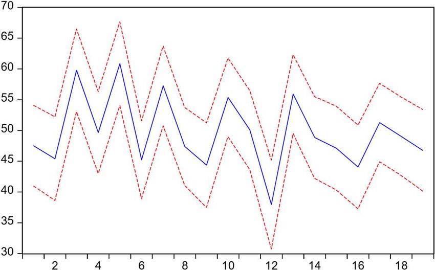
Thus, we conclude that with 95% confidence level, the vote share of Republican Party
candidate Donald Trump will be 46.74% with standard error of ±2.638%. Summarizing the
results on the basis of the above model we conclude that Democratic Party candidate Mr. Joe
Biden will win the 2020 US Presidential election.
± 2 S.E.
VOTEF
FIGURE 1- Forecasted vote percentage for all the observations
CONCLUSION
The proposed model predicts the victory of the Republican party candidate Mr. Joe Biden in
the 2020 U.S. Presidential election. The model was also tested for predicting the 2016 U.S.
Presidential election successfully, with the vote share of the incumbent party being 49.16%,
which is quite close to the actual vote percentage (48.2%) received by the Democratic party
candidate Hilary Clinton.
The suggested model highlights the importance of non-economic variables for the U.S.
Presidential outcome forecast. The analysis of economic variables depicts the significance of
the growth of the economy as the only significant variable leaving aside the annual inflation,
exchange rate, unemployment rate, gold price, and oil prices. On the other hand, while
developing the final model, it turns out that the only significant factors are the non-economic
factors - The Gallup job approval rating in June of the election year, the period of running of
the incumbent party, and the scandal rating.REFERENCES
1. Lewis-Beck, M. S. & Rice, T. W. (1982).Presidential Popularity and Presidential Vote.
The Public Opinion Quarterly, 46 4, 534-537.
2. Fair, R. C. (1978). The effect of economic events on votes for president. Review of
Economics and Statistics, 60, 159-173 Fair, R.C. (2016). Vote-Share Equations:
November 2014 update, retrieved from
http://fairmodel.econ.yale.edu/vote2016/index2.htm
3. Silver, N. (2011). On the Maddeningly Inexact Relationship Between Unemployment and
Re-Election, retrieved from
http://fivethirtyeight.blogs.nytimes.com/2011/06/02/onthemaddeningly- inexact-
relationship-between-unemployment-and-re-election/.
4. Jérôme, Bruno & Jérôme -Speziari, Veronique. (2011). Forecasting the 2012 U.S.
Presidential Election: What Can We Learn from a State Level Political Economy Model.
In Proceedings of the APSA Annual meeting Seattle, September 1-4 2011
5. Cuzán, A. G., Heggen R.J., & Bundrick C.M. (2000). Fiscal policy, economic conditions,
and terms in office: simulating presidential election outcomes. In Proceedings of the World
Congress of the Systems Sciences and ISSS International Society for the Systems
Sciences, 44th Annual Meeting, July 16–20, Toronto, Canada.
6. Abramowitz A. I. (1988). An Improved Model for Predicting the Outcomes of Presidential
Elections. PS: Political Science and Politics, 21 4, 843-847
7. Lichtman, A. J. (2005). The Keys to the White House. Lanham, MD: Lexington Books.
Lichtman, A. J. (2008). The keys to the white house: An index forecast for 2008.
International Journal of Forecasting, 24, 301–309.
8. Erikson, R. S., and Wlezien, C. (1996). Of time and presidential election forecasts. PS:
Political Science and politics, 31, 37-39
9. Hibbs D. A. (2000). Bread and Peace voting in U.S. presidential elections. Public Choice,
104, 149–180. Hibbs, Douglas A. (2012). Obama’s Re-election Prospects Under ‘Bread
and Peace’ Voting in the 2012 US Presidential Election. Retrieved from:
http://www.douglashibbs.com/HibbsArticles/HIBBS_OBAMA-REELECT-
31July2012r1.pdf.
10. Sinha, P. and Bansal, A.K. (2008). Hierarchical Bayes Prediction for the 2008 US
Presidential Election. The Journal of Prediction Markets, 2, 47-60.
11. Seigelman, L., (1979). Presidential popularity and presidential elections. Public Opinion
Quarterly, 43, 532-34.
12. Fair, R. C. (2002). Predicting Presidential Elections and Other Things. Stanford: Stanford
University Press.13. Mueller J.E. (1970), Presidential Popularity from Truman to Johnson. The American
Political science review, 64, 18-34. 22.
14. Lichtman, A. J., and Keilis-Borok, V. I. (1981). “Pattern Recognition Applied to
Presidential Elections in the United States, 1860-1980: Role of Integral Social, Economic
and Political Traits,” Proceedings of the National Academy of Science, Vol. 78, No. 11,
pp. 72307234
15. Tufte, E. R. (1975). Determinants of the Outcomes of Midterm Congressional Elections.
American Political Science Review, 69, 812-26.
16. Usinflationcalculator.com (2020). Current US Inflation Rates: 2009-2020. Retrieved from
https://www.usinflationcalculator.com/inflation/current-inflation-
rates/#:~:text=The%20annual%20inflation%20rate%20for,published%20on%20October
%2013%2C%202020
17. Bureau of Labor Statistics (2020). Civilian Unemployment Rate. Retrieved from
https://www.bls.gov/charts/employment-situation/civilian-unemployment-rate.htm
18. Federal Reserve Bank of St. Louis (2020). Real GDP Per Capita. Retrieved from
https://fred.stlouisfed.org/series/A939RX0Q048SBEA#0
19. National Mining Association. Historical Gold Prices, 1833 to Present. Retrieved from
https://nma.org/wp-content/uploads/2019/02/his_gold_prices_1833_pres_2019.pdf
20. Inflationdata.com (2020). Historical Crude Oil Price (Table). Retrieved from
https://inflationdata.com/articles/inflation-adjusted-prices/historical-crude-oil-prices-
table/
21. Federal Reserve Bank of St. Louis, retrieved from
https://fred.stlouisfed.org/series/EXUSUK
22. Gallup Presidential Poll. (2016). Presidential Job Approval Centre. Retrieved from
https://news.gallup.com/poll/203198/presidential-approval-ratings-donald-trump.aspx
23. DisasterCenter.com (2020). US Crime Rates 1960-2019. Retrieved from
http://www.disastercenter.com/crime/uscrime.htm
24. History, Art and Archives, US House of Representatives (2020). Election Statistics, 1920
to Present. Retrieved from https://history.house.gov/Institution/Election-
Statistics/Election-Statistics/
25. Federal Election Commission (2020). Campaign Finance Data (2020) Biden for President.
Retrieved from https://www.fec.gov/data/committee/C00703975/?tab=spending
26. Federal Election Commission (2020). Campaign Finance Data Donald J. Trump. Retrieved
from https://www.fec.gov/data/committee/C00580100/?tab=spending&cycle=202027. BBC.com (2020). Trump impeachment: The short, medium and long story. Retrieved from
https://www.bbc.com/news/world-us-canada-49800181APPENDIX
Table 8: Popular and Electoral Votes received by Incumbent party candidates
Source: uselectionatlas.org
Year Popular vote Electoral vote
952 44.33% 16.80%
1956 57.37% 86.10%
1960 49.55% 40.80%
1964 61.05% 90.30%
1968 42.72% 35.50%
1972 60.67% 96.70%
1976 48.01% 44.60%
1980 41.01% 9.10%
1984 58.77% 97.60%
1988 53.37% 79.20%
1992 37.45% 31.20%
1996 49.23% 70.40%
2000 48.38% 49.40%
2004 50.73% 53.20%
2008 45.60% 32.20%
2012 51.01% 61.70%
2016 48.02% 42.20%Table 9: Scandals during Presidential Terms and the Corresponding Ratings
Year Incumbent President Scandals Rating
1952 Harry S. Truman • Continuous accusations of spies in the US Govt. 1
• Foreign policies: Korean war, Indo China war
White house renovations
• Steel and coal strikes
• Corruption charges
1956 Dwight D. • None 0
Eisenhower
1960 Dwight D. • U-2 Spy Plane Incident 1
Eisenhower • Senator Joseph R. McCarthy Controversy
• Little Rock School Racial Issues
1964 John F. Kennedy • Extra-marital relationship
0
Lyndon B. Johnson • None
1968 Lyndon B. Johnson • Vietnam war 1
• Urban riots
• Phone Tapping
1972 Richard Nixon • Nixon Shock 0
1976 Richard Nixon • Watergate
2
Gerald Ford • Nixon Pardon
1980 Jimmy Carter • Iran hostage crisis
• 1979 energy crisis 1
• Boycott of the Moscow Olympics
1984 Ronald Reagan • Tax cuts and budget proposals to expand military 0
spending
1988 Ronald Reagan • Iran-Contra affair 1
• Multiple corruption charges against high ranking
officials
1992 George H W Bush • Renegation on election promise of no new taxes 1
• "Vomiting Incident"
1996 Bill Clinton • Firing of White House staff 1
• "Don't ask, don't tell” policy
2000 Bill Clinton • Lewinsky Scandal 2
2004 George W Bush • None 0
2008 George W Bush • Midterm dismissal of 7 US attorneys 1
• Guantanamo Bay Controversy and torture2012 Barack Obama • None 0
2016 Barack Obama • None 0
2020 Donald Trump • Ukraine Impeachment Scandal Tax 1
• EvasionTable 10: Gallup Ratings
Source: Gallup Presidential Poll (2020)
Year Incumbent President June Gallup Rating Average Gallup
Rating
1952 Harry S. Truman 31.5 36.5
1956 Dwight D. 72 69.6
Eisenhower
1960 Dwight D. 59 60.5
Eisenhower
1964 Lyndon B. Johnson 74 74.2
1968 Lyndon B. Johnson 41 50.3
1972 Richard Nixon 57.5 55.8
1976 Gerald Ford 45 47.2
1980 Jimmy Carter 33.6 45.5
1984 Ronald Reagan 54 50.3
1988 Ronald Reagan 50 55.3
1992 George H W Bush 37.3 60.9
1996 Bill Clinton 55 49.6
2000 Bill Clinton 57.5 60.6
2004 George W Bush 48.5 62.2
2008 George W Bush 29 36.5
2012 Barack Obama 46.4 49.0
2016 Barack Obama 51.6 48.0
2020 Donald Trump 38 41Table 11: Mid-Term Election Results (1948-2018);
Source: Office of the Clerk (US)
Mid Term Senate
Election House Seats House Seats Senate Midterm
Year Incumbent Party Year D R Result D R Result Values
1948 263 171 54 42
1952 Democratic 1950 234 199 1 48 47 1 1
1952 213 221 46 48
1956 Republican 1954 232 203 -1 48 47 -1 -1
1956 234 201 49 47
1960 Republican 1958 283 153 -1 64 34 -1 -1
1960 262 175 64 36
1964 Democratic 1962 258 176 1 67 33 1 1
1964 295 140 68 32
1968 Democratic 1966 248 187 1 64 36 1 1
1968 243 192 58 42
1972 Republican 1970 255 180 -1 54 44 -1 -1
1972 242 192 56 42
1976 Republican 1974 291 144 -1 61 37 -1 -1
1976 292 143 61 38
1980 Democratic 1978 277 158 1 58 41 1 1
1980 242 192 46 53
1984 Republican 1982 269 166 -1 46 54 1 -0.63
1984 253 182 47 53
1988 Republican 1986 258 177 -1 55 45 -1 -0.63
1988 260 175 55 45
1992 Republican 1990 267 167 -1 56 44 -1 -1
1992 258 176 57 43
1996 Democratic 1994 204 230 -1 48 52 -1 -1
1996 207 226 45 55
2000 Democratic 1998 211 223 -1 45 55 -1 -1
2000 212 221 50 50
2004 Republican 2002 204 229 1 48 51 1 1
2004 202 232 44 55
2008 Republican 2006 233 202 -1 49 49 0 -0.82
2008 256 178 55 41
2012 Democratic 2010 193 242 -1 51 47 1 -0.63
2012 200 234 53 45
2016 Democratic 2014 188 247 -1 44 54 1 -0.63
2020 Republican 2016 194 241 -1 46 52 1 -0.632018 235 199 45 53
Table 12: Economic Data
Source: a: Bureau of Labour Statistics; b: usinflationcalculator.com; c: National Mining
Organization; d: inflationdata.com; e: Federal Bank of St. Louis

                                                        Gold Price     Oil       Ex. rate
  Year  Unemploymenta Inflationb Gold_price_indexc      ($/ounce)c   Pricesd   (USD/GBP)e
   1952         3.07         7.9                             34.6     26.92          2.79
    1956             4.03      -0.4                 1       34.99     27.92          2.80
    1960             5.13       0.7                 1       35.27     25.41          2.80
    1964             5.47       1.3                 0        35.1     24.95          2.79
    1968             3.73       3.1                 1       39.31     23.55          2.39
    1972             5.77       4.4                 1       58.42     22.21          2.57
    1976             7.73       9.1                 1      124.74      59.4          1.76
    1980              6.3      11.3                 1         615     117.3          2.34
    1984             7.87       3.2                 0         361     71.41          1.38
    1988              5.7       3.6                 1         437     32.48          1.78
    1992             7.37       4.2                 0      343.82     35.39          1.86
    1996             5.53       2.8                 1      387.81     33.63          1.54
    2000             4.03       2.2                 0      279.11     41.02          1.51
    2004              5.7       2.3                 1      409.72     51.39          1.83
    2008               5        2.8                 1      871.96    109.25          1.97
    2012             8.27       3.2                 1    1668.98      97.17          1.56
    2016             4.93       0.1                 0    1250.74      39.02          1.42
    2020             3.83       1.8                 1      1392.6     39.42          1.25
Table 13: Non-Economic Data
Source: a: http://www.disastercenter.com/crime/uscrime.html ; b: Wikipedia; c: Wikipedia; d:
Federal Election Commission (www.fec.gov)
Incumbent President Campaign spending
Year Crime ratea Runningb Period of powerc Indexd
1952 0 1 0
1956 1 0 2
1960 0 1 1
1964 1998.35 1 0 0
1968 2624.4 0 1 0
1972 3549.85 1 0 2
1976 4566.18 1 1 1
1980 5267.7 1 0 0
1984 5646.73 1 0 1
1988 5317.2 0 1 1
1992 5780.83 1 1 0
1996 5448.25 1 0 1
2000 4724.23 0 1 0
2004 4119.85 1 0 1
2008 3854.08 0 1 0
2012 3444.35 1 0 1
2016 3049.85 0 1 1
2020 2672.35 1 0 0You can also read