Predicting Taxi Pickups in New York City
←
→
Page content transcription
If your browser does not render page correctly, please read the page content below
Predicting Taxi Pickups in New York City
Josh Grinberg, Arzav Jain, Vivek Choksi
Final Paper for CS221, Autumn 2014
ABSTRACT
There were roughly 170 million taxi rides in New York City in 2013. Exploiting an understanding of taxi
supply and demand could increase the efficiency of the city’s taxi system. In this paper, we present a few
different models to predict the number of taxi pickups that will occur at a specific time and location in New
York City; these predictions could inform taxi dispatchers and drivers on where to position their taxis. We
implemented and evaluated three different regression models: linear least-squares regression, support vector
regression, and decision tree regression. Experimenting with various feature sets and performing grid-search
to tune hyperparameters, we were able to achieve positive results. Our best-performing model, decision tree
regression, achieved a root-mean-square deviation of 33.5 and coefficient of determination (R2) of 0.99, a
significant improvement over our baseline model’s root-mean-square-deviation of 146 and R2 of 0.73.
I. INTRODUCTION AND MOTIVATION Chris Whong [1]. The data associates each taxi ride
The ability to predict taxi ridership could present with information including date, time, and location of
valuable insights to city planners and taxi dispatchers pickup and drop-off.
in answering questions such as how to position cabs A small number of taxi pickups in this dataset
where they are most needed, how many taxis to originate from well outside the New York City area. In
dispatch, and how ridership varies over time. Our order to constrain our problem to New York City as
project focuses on predicting the number of taxi well as to reduce the size of our data given our limited
pickups given a one-hour time window and a location computational resources, we only consider taxi trips
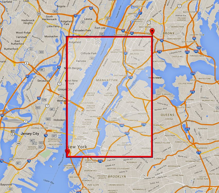
within New York City. This project concept is inspired that originate somewhere within the 28-square-mile
by the MIT 2013-2014 Big Data Challenge, which rectangular region that encloses Manhattan as shown
proposed the same problem for taxicabs in Boston. and defined in Figure 1 below. To further limit the
The problem is formulated in terms of the following size of our data, we only consider taxi rides in the
inputs and outputs: months of January through April.
Input.
Date, one-hour time window, and latitude and
longitude coordinates within New York City.
e.g. “17 March 2013, from 5 PM to 6 PM, at coordinates
(40.75, -73.97)”
Output.
Predicted number of taxi pickups at the input time and
location.
e.g. “561.88 pickups”
II. METHODOLOGY
A. Data Management
We use a dataset detailing all ~170 million taxi trips in
New York City in 2013, as provided by the Freedom
of Information Law and hosted on the website of Figure 1. We only consider taxi rides in the portion of
1 All taxi data is accessible at: chriswhong.com/open-
data/foil_nyc_taxi.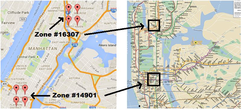
New York City between latitudes 40.70o to 40.84o and        C. Feature Extraction
longitudes -74.02o to -73.89o. This rectangular region      Below is a list of feature templates we use to extract
encloses the city’s densest areas: Manhattan, part of       features from each data point, along with a rough
Queens, and part of the Bronx.                              intuition as to why these features might be predictive.
We divide our rectangular region of New York City           1. Zone ID. We expect location to be highly
into a grid of 0.01o x 0.01o squares called zones. Each        predictive of taxi traffic.
zone roughly corresponds to 1km x 1km region.
                                                            2. Hour of day ∈ [0, 23]. We expect overall NYC taxi
For ease of querying and aggregation, we store the             ridership to follow a daily cycle.
data in a MySQL database hosted on Amazon RDS.              3. Day of week ∈ [0, 6]. We expect day of week to
In order to put the raw data into the same form as our         correlate with taxi traffic.
input to the problem, we group the raw taxi data by         4. Zone and hour of day combined. Daily patterns in
time (at the granularity of an hour) and zone, count           ridership may be different in different zones. For
the total number of pickups for each time-zone                 example, at 12 PM, taxi traffic may drop in
combination, and store these aggregated values as data         residential zones (because people are at work) but
points to be used for training and testing. For instance,      increase in commercial zones (because workers go
one row in our aggregated pickups table is “2013-03-           out to lunch). Combining zone and hour of day
05 15:00:00, 15704, 811”, representing 811 pickups in          would capture such an inter-feature dependency.
Zone #15704 on March 5, 2013 between 3 PM and 4             5. Zone, day of week, and hour of day combined. Even
PM local time. In total, our data set consists of              within a specific zone, the same hour of day may
482,000 such data points.                                      have a different effect during different days of the
                                                               week.
B. Evaluation                                               6. Hourly precipitation, measured in hundredths of an
In order to evaluate the performance of our model, we          inch, provided by the National Climatic Data
split the data into a training set and testing set, where      Center [2], and discretized into 3 buckets
the training examples are all ordered chronologically          representing no rain, less than 0.1 inches of rain in
before the testing examples. This configuration                an hour, and at least 0.1 inches of rain in an hour.
mimics the task of predicting future numbers of taxi           We expect precipitation to increase taxi ridership,
pickups using only past data.                                  since in rainy weather people may prefer taking
                                                               taxis to walking or taking public transportation.
We considered using a few different error metrics to        7. Zone, day of week and hourly precipitation combined.
evaluate our predictions: RMSD, mean absolute error,           Rainfall may have a different impact on different
and a root-mean-square percent deviation. We                   zones at different times of the day.
ultimately chose RMSD because it favors consistency
and heavily penalizes predictions with a high deviation     All features defined by the feature templates above are
from the true number of pickups.                            binary.       For       example,        the      feature
                                                            “ZONE=15403_DAY=5_HOUR=13”, derived from
From the point of view of a taxi dispatcher, any large      feature template #5 in the list above, has a value of 1
mistake in gauging taxi demand for a particular zone        only if the data point represents a taxi pickup in Zone
could be costly ‒ imagine sending 600 taxis to a zone       #15403 on Saturday (day 5) between 1 PM and 2 PM.
that only truly requires 400. This misallocation results
in many unutilized taxis crowded in the same place,         We did not experiment with quadratic or any other
and should be penalized more heavily than dispatching       polynomial operations on our numerical features
6 taxis to a zone that only requires 4, or even             because we did not expect any polynomial relationship
dispatching 6 taxis to 100 different zones that only        between our features and the number of taxi pickups.
require 4 taxis each. RMSD most heavily penalizes
such large misallocations and best represents the
quality of our models’ predictions.

In comparing the results between our different
models, we also report the R2 value (coefficient of
                                                            2 All weather data is available at: ncdc.noaa.gov. The
determination) in order to evaluate how well the
                                                            weather data we use in our project was observed from the
models perform relative to the variance of the data set.
                                                            New York Belvedere Observation Tower in Central Park.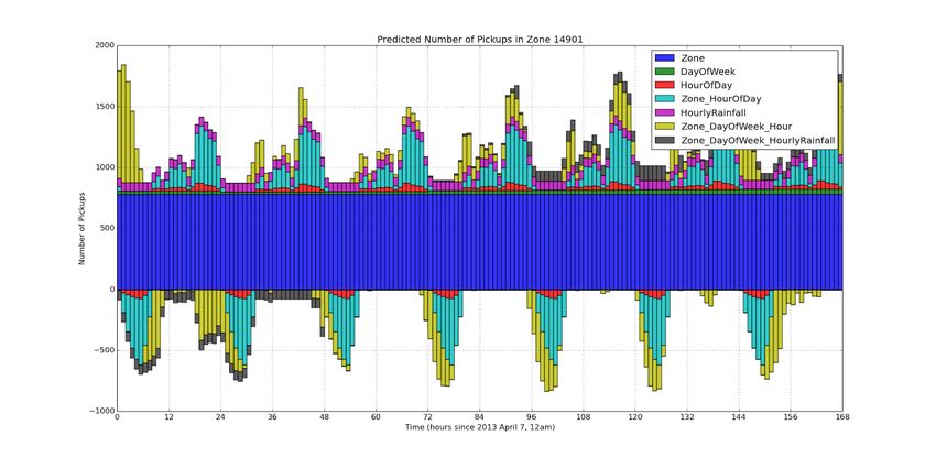
D. Regression Models                                       obtained by training on the first 70% of the data
Baseline Model.                                            points (January 1 through March 28) and testing on
Our baseline model predicts the number of pickups on       the remaining 30% (March 29 through April 30). The
a test data point at a given zone as the average number    hyperparameters used for each model are determined
of pickups for all training data points in that zone.      using grid-search over select parameter values, and the
                                                           best features to use for each model are determined
To improve upon this baseline, we experiment with          through experimentation.
three different regression models described below. We
use the Python module scikit-learn to apply our                       Model           Root-mean-    Coef. of
regression models.                                                                      square   Determination
                                                                                       Deviation      (R2)
Linear least-squares regression.
                                                           Baseline                     145.78        0.7318
The linear regression model allows us to exploit linear
patterns in the data set. This model is an appealing       Linear Least-Squares
first choice because feature weights are easily            Regression                   40.74         0.9791
                                                           (Feature Set #2)
interpretable and because stochastic gradient descent
runs efficiently on large datasets. We choose squared      Support Vector
loss (square of the residual) as our objective function    Regression
                                                                                        79.77
                                                           (Feature Set #2; trained                   0.9197
in stochastic gradient descent because minimizing it
                                                           on 50K randomly selected
directly relates to minimizing our error metric, root-
                                                           training examples)
mean-square-deviation.
                                                           Decision Tree Regression
                                                                                        33.47         0.9858
Epsilon Support Vector Regression.                         (Feature Set #1)
Our feature templates produce a large number of            Table 1. Best results for each model. The feature sets
features; for example, the feature template                are defined in the Table 2 below.
“Zone_DayOfWeek_HourOfDay” alone produces
179!zones!×!7!days!per!week!×!24!hours!per!day →                             Zone
30,072 binary features. We choose to include support                         HourOfDay
                                                            Feature Set #1
                                                                             DayOfWeek
vector regression since support vector machines
                                                                             HourlyRainfall
perform well with many sparse features and can derive
                                                                             Zone
complex non-linear boundaries depending on the                               HourOfDay
choice of the kernel.                                       Feature Set #2   DayOfWeek
                                                                             Zone_HourOfDay
Decision Tree Regression.                                                    Zone_DayOfWeek_HourOfDay
The decision tree regression model is both easy-to-                          Zone
interpret and capable of representing complex decision                       HourOfDay
boundaries, thus complementing our other chosen                              DayOfWeek
                                                            Feature Set #3
models. We run the decision tree regression model on                         Zone_HourOfDay
a reduced feature set (Feature Set #1 as defined in                          Zone_DayOfWeek_HourOfDay
Table 2) that excludes feature templates containing                          Zone_DayOfWeek_HourlyRainfall
combination features. We do this for two reasons: (1)      Table 2. List of the feature templates that compose
training the decision tree model using all 36,649 binary   each feature set.
features contained in Feature Set #2 (defined in Table     A. Hyperparameters
2) is prohibitively computationally expensive, since
                                                           Below, we discuss the results of grid search for each
each new node in the decision tree must decide on
                                                           model.
which feature to split, and (2) combination features
essentially represent the AND operation applied to         Linear
multiple binary features; since this AND operation is      The three hyperparameters tested using grid search
naturally represented by paths in the decision tree,       were the number of iterations of stochastic gradient
including combination features would be redundant.         descent, !! , and p, where !! and p are parameters of
                                                                                                      !
III. RESULTS                                               the inverse-scaled learning rate ! = ! !! . These
                                                                                                      !
                                                           parameters are important to the model because they
Table 1 summarizes the best results for each model,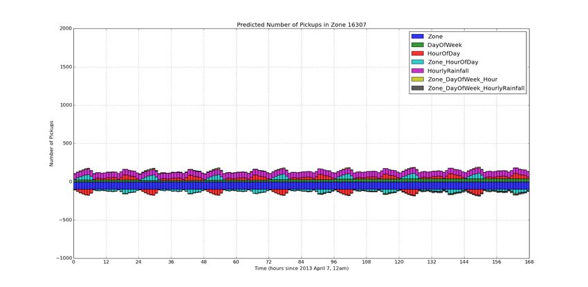
control the extent to which the model converges to an
optimal value. The model converged to an optimum             Feature Set       Root-mean-           Coef. of
R2 value of about 0.98 using 8000 iterations of                                  square          Determination
stochastic gradient descent and parameter values                                Deviation             (R2)
!! = 0.2, and p = 0.4.                                      Feature Set #1
                                                                                  138.05              0.7595
                                                            (Basic features)
Support Vector Regression
                                                            Feature Set #2
Because training support vector regression on large
                                                            (Basic + feature       40.07              0.9797
data set sizes is computationally expensive, we were
                                                            combinations)
only able to grid-search one parameter, the
                                                            Feature Set #3
regularization parameter C. Our model performed best
                                                            (Basic + feature
with a high C value of 1 x 10⁷, indicating that lower                              40.74              0.9791
                                                            combinations
values of C underfit the data and resulted in too few
                                                            + precipitation)
support vectors. We used a radial basis function kernel
                                                            Table 3. Results of linear regression using different
in order to introduce nonlinearity; using a nonlinear
                                                            feature sets.
further increases the computation time with LibSVM.
In order to lower computation time, we ran support          Analysis of feature weights
vector regression on a reduced training set size of         In order to better understand the relative importance
50,000 data points (as opposed to ~337,000 data             of our feature templates, we use the linear regression
points for the other models). For reference, training       model to generate stacked bar charts of all feature
the support vector regression using the full training set   weights that are used to make predictions over the
did not complete in even 8 hours of running on a            course of a week. That is, at each hour interval in a
Stanford Barley machine using 4 cores. It is likely that    given zone, we stack the weights of all the features
support vector regression performed much worse than         whose values are 1 for that data point. The predicted
the other models because of this relatively small           number of taxi pickups at a given hour can be
training set size, achieving a root-mean-square             visualized by adding the heights of all the positive
deviation value of 79.77.                                   feature weights and subtracting the heights of all the
                                                            negative feature weights. Since all features are binary,
Decision Tree Regression                                    the feature weights map directly to the number of taxi
The two hyperparameters tuned were the maximum              pickups. In other words, if the weight of feature
depth of the tree and the minimum number of                 “ZONE=16304” is 126, then this feature contributes
examples that a leaf node must represent. These two         +126 pickups to the total predicted number of
parameters are important to the model because they          pickups for this data point.
balance overfitting and underfitting. Of the values we
swept, our model performed best with a minimum of
2 examples per leaf and a maximum tree-depth of 100.
With greater tree-depths, the model achieved the same
performance on the test set, suggesting that tree-
depths greater than 100 contribute to overfitting.

B. Feature Analysis
Experiments with different feature sets
In order to determine which feature sets produce the
best results, we define three feature sets (see Table 2
above). Below are the results obtained running the
linear regression model on each feature set.

We observe that feature combinations significantly
improve results, as expected. Also, counter to our
intuitions, weather features do not improve results
(Table 3).
Figure 2. Feature weights used to make predictions at 2 PM in Zone #14901 has a higher feature weight
each hour over the course of a week (April 7, 2013 relative to other times of day than does 2PM in Zone
through April 13, 2013), for two different zones in New
#16307.
York City, one busy (Zone #14901, top) and one quiet
(Zone #16307, bottom). The weights of the weather feature templates present
The feature weight plots in Figure 2 validate many of interesting and nuanced results. It rained heavily
the intuitions we used to pick features. For example, between April 11 and April 13 (hours 96 through 168).
we notice small daily cycles common to both zones; Despite this period of intense rain, the weights of the
this justifies the importance of the ‘HourOfDay’ ‘HourlyRainfall’ features (magenta series) are roughly
feature template (red series). These feature weights constant throughout the week—this suggests that
represent the daily taxi traffic cycles in New York City rainfall has little effect on taxi ridership in New York
across all zones. Furthermore, the ‘Zone_HourOfDay’ City overall. Now, consider zone-specific effects of
feature weights (cyan series) validate our intuition that rain. From the plots, we see that
daily taxi traffic patterns may vary by zone: notice that ‘Zone_DayOfWeek_HourlyRainfall’ features predicthigher taxi ridership during heavy rain in Zone
#14901, but slightly lower taxi ridership during heavy
rain in Zone #16307. As depicted in the maps in
Figure 3 below, Zone #14901 is much more densely
populated than Zone #16307 and contains multiple
subway stops. Perhaps people in Zone #14901 opt for
taxis as opposed to public transportation when it is
raining more than people in Zone #16307. As we had
suspected, rain appears to have different effects in
different zones, validating the usefulness of our
combination feature template.
Figure 3. Zones #14901 and #16307 on a road map and
a NYC Subway map.
C. Model Analysis
In order to visualize how well the models perform, we
plot the true versus predicted number of pickups for
each data point in the test set in Figure 4.
Figure 4. Predicted versus true number of pickups
The scatter plots in Figure 4 suggest that the linear using least-squares linear regression (top) and decision
regression and decision tree regression models tree regression (bottom).
perform well on the test set. Most predictions lie close
The baseline model performs very poorly by
to the true values. The data points straddle the unit-
comparison. This is unsurprising, since the baseline
slope line evenly, signifying that the models do not
naively predicts the same value for all data points in a
systematically underestimate or overestimate the
given zone, as shown by the horizontal streaks of
number of taxi pickups. For both models, as expected,
points in Figure 5.
absolute prediction error increases as the true number
of pickups increases. This effect can be visualized as a
cone-shaped region extending outward from the origin
within which the data points fall. The error plot for
support vector regression (not shown) looks roughly
the same, but with more dispersion of data points.
Figure 5. Predicted versus true number of pickups
using the baseline model.Analysis of Decision Tree Regression on zone provides the most information gain. Once a
Of all of our models, decision tree regression data point’s zone is ascertained, it is next asked for its
performed best, achieving an RMSD value of 33.47. In hour of day, then day of week, and finally amount of
order to quantify bias, variance, and the degree to precipitation. This ordering of feature templates by
which the model has converged, we plot learning descending information gain is consistent with the
curves, shown below in Figure 6. The learning curves relative weights of features produced by the linear
indicate that the decision tree regression model regression model, shown in Figure 2: zone-based
converges using a training set size of as few as 100,000 features are most informative, and weather-based
training examples. Using greater than 100,000 training features are least informative.
examples, the test and training R2 scores are practically
identical and well above 0.97, indicating that the model
achieves both low bias and low variance.
Figure 7. Subsection of the final trained decision tree.
One possible reason this model outperforms linear
regression and support vector regression is that
although it is run on a smaller feature set, paths within
the tree are able to represent the combination of (that
is, the AND operation applied to) any number of
features in Feature Set #1. For example, the decision
tree regression model is able to capture the effect of
rainfall on taxi pickups specifically on Sundays at 4am
in Zone #15102 (as shown in rightmost paths of the
above tree), whereas the other models cannot easily
capture such dependencies between features (short of
combining all features together). Perhaps it is because
these features in Feature Set #1 are highly dependent
upon one another that the decision tree regression
performs best of all the models we tried.
IV. CONCLUSIONS AND FUTURE WORK
Figure 6. Learning curves for decision tree regression, Conclusion
showing up to 70,000 training data points (top) and up Overall, our models for predicting taxi pickups in New
to ~337,000 training data points (bottom).
York City performed well. The decision tree regression
The tree diagram in Figure 7 shows a subsection of the model performed best, likely due to its unique ability
trained decision tree. Since all of our features are to capture complex feature dependencies. The
binary, each node in the tree represents one of the 206 decision tree regression model achieved a value of
features in Feature Set #1 upon whose value the data 33.47 for RMSD and 0.9858 for R2 ‒ a significant
can be split. Evaluating a test data point using a improvement upon the baseline’s values of 145.78 for
decision tree can be imagined as asking the data point RMSD and 0.7318 for R2. Our experiments, results,
true-or-false questions until a leaf node is reached. As and error analysis for the most part supported our
the tree diagram begins to show, the first question that intuitions about the usefulness of our features, with
our tree asks is what zone the data point resides in, the exception of the unexpected result that weather
since the decision tree has determined that branching features did not improve model performance. A modelsuch as ours could be useful to city planners and taxi V. ACKNOWLEDGMENTS dispatchers in determining where to position taxicabs We earnestly thank Professor Percy Liang and the and studying patterns in ridership. entire CS221 teaching staff for equipping us with the Future work conceptual tools to complete this project. We give Predictions for arbitrary zones and time intervals special thanks to Janice Lan for her thoughtful Currently, our model predicts pickups only for pre- feedback on our project as it matured over the course defined zones and 1-hour time intervals. We could of the quarter. extend our model to predict the number of taxi pickups in arbitrarily sized zones and time intervals. We could do this by training our model using very small zones and time intervals. In order to predict the number of pickups for a larger region and time interval, we could sum our granular prediction values across all mini-zones in the specified region and all mini-time-intervals in the desired time interval. Neural network regression. We may be able to achieve good results using a neural network regression, since neural networks can automatically tune and model feature interactions. Instead of manually determining which features to combine in order to capture feature interactions, we could let the learning algorithm perform this task. One possible instance of features interacting in the real world could be that New Yorkers may take taxi rides near Central Park or when it is raining, but not when they are near Central Park and it is raining, since they may not visit the park in bad weather. Neural networks could be promising because they can learn nonlinearities automatically, such as this example of an XOR relationship between features. In addition to our three core regression models, we implemented a neural network regression model using the Python library PyBrain. However, we would need more time to give the neural network model due consideration, so we list it here as possible future work. Clustering feature template. In order to find non-obvious patterns across data points, we could use unsupervised learning to cluster our training set. The clustering algorithm could use features such as the number of bars and restaurants in a given zone, or distance to the nearest subway station. The cluster in which each data point falls could then serve as an additional feature for our regression models, thereby exploiting similar characteristics between different zones for learning.
You can also read