FOREX Trend Classification using Machine Learning Techniques
←
→
Page content transcription
If your browser does not render page correctly, please read the page content below
Recent Researches in Applied Informatics and Remote Sensing

    FOREX Trend Classification using Machine Learning Techniques
                 AREEJ ABDULLAH BAASHER, MOHAMED WALEED FAKHR
                               Computer Science Department
                         Arab Academy for Science and Technology
                                      Cairo, EGYPT
                        baasher_areej@yahoo.com, waleedf@aast.edu

Abstract :- Foreign Currency Exchange market                   In time series analysis, it is always a challenge to
(Forex) is a highly volatile complex time series for           determine the required history window used by the
which predicting the daily trend is a challenging              classification or forecasting system to do its
problem. In this paper, we investigate the prediction          prediction. In this paper, we have taken an approach
of the High exchange rate daily trend as a binary              of providing features from multiple time windows
classification problem, with uptrend and downtrend             ranging from one day up to 30 days. This of course
outcomes. A large number of basic features driven              results in a number of features larger than using a
from the time series data, including technical analysis        single time window. Processing of the raw time
features are generated using multiple history time             domain daily values is done to produce the basic
windows. Various feature selection and feature                 features used in the feature selection and extraction
extraction techniques are used to find best subsets for        steps. This processing involves calculation of
the classification problem. Machine learning systems           technical analysis and other time and frequency
are tested for each feature subset and results are             domain features over multiple time windows with a
analyzed. Four important Forex currency pairs are              total of 81 basic features. Our approach is to let
investigated and the results show consistent success in        feature selection and feature extraction techniques
the daily prediction and in the expected profit.               find the best set of features for the classification task.
                                                               Feature selection techniques choose a subset of the
  Keywords: - Technical analysis, Feature selection,           basic features while feature extraction techniques find
Feature extraction, Machine-learning techniques,               features in new projected spaces. In this paper, two
Bagging Trees, SVM, Forex prediction.                          feature selection and six feature extraction techniques
                                                               are used which all aim at finding feature subsets to
                                                               enhance the classification performance.
    1 Introduction                                               For each feature subset, three supervised machine
                                                               learning classifiers are used, namely, radial basis
This paper is about predicting the Foreign Exchange            function neural network (RBF), multilayer perceptron
(Forex) market trend using classification and machine          neural network (MLP) and support vector machine
learning techniques for the sake of gaining long-term          (SVM). This gives a large array of different feature
profits. Our trading strategy is to take one action per        subsets and different classifiers. Comparison between
day, where this action is either buy or sell based on          these different systems is done based on two factors.
the prediction we have. We view the prediction                 The first is the percentage classification performance
problem as a binary classification task, thus we are           on the test data. The second is a novel function we
not trying to predict the actual exchange rate value           call the percentage normalized profit (PNP), which
between two currencies, but rather, if that exchange           represents the ratio between the accumulated profits
rate is going to rise or fall. Each day there are four         using the predicted trends versus the accumulated
observed rates, namely, the "Open", "Close", "Low"             profit using perfect predictions along the duration of
and "High". In this work, we focus on predicting the           the test period. We have selected four Forex pairs
direction of the "High".                                       which are namely the USD/YEN, USD/EGP,
Forex daily exchange rate values can be seen as a              EURO/EGP and EURO/SAR (where EGP is the
time series data and all time series data forecasting          Egyptian pound and SAR is the Saudi Riyal). The
and data mining techniques can be used to do the               remaining of this paper is organized as follows.
required classification task.                                  Section 2 discusses the nature of the Forex data, and
                                                               the most prominent approaches used in the literature

    ISBN: 978-1-61804-039-8                               41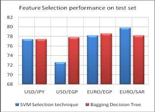
Recent Researches in Applied Informatics and Remote Sensing

to represent this data. In particular, the Technical               2.2 FOREX Prediction Review
Analysis (TA) approach is explained and the relevant
TA features used in this work are outlined. Section III         Economic time series prediction techniques are
focuses on the particular features used in this work,          classified into two main categories; namely,
where we have combined the ideas of the TA and                 techniques that try to predict the actual value of the
some signal analysis ideas, over multiple window               rate exchange or the actual returns value and
sizes to get 81 basic features.                                techniques that try to predict the trend direction
   Section 4 outlines the feature selection and feature        (uptrend, downtrend and sideways).
extraction techniques used in this work. For feature           Exchange rates prediction is one of the most
selection, an SVM-based, and a Bagging decision tree           challenging applications of modern time series
ensemble methods are used. For feature extraction              forecasting. The rates are inherently noisy, non-
five methods are used, namely, PCA per class method            stationary and deterministically chaotic [1]. One
(PCAClass), linear discriminant analysis between               general assumption is made in such cases is that the
clusters and class's method (LDA Cluster/Class), and           historical data incorporate all of those behaviors. As a
between pairs of clusters (LDA Cluster/Cluster),               result, the historical data is the major player in the
maximally collapsing metric learning algorithm                 prediction process [1, 2].
(MCML) and neighborhood components analysis                    For more than two decades, Box and Jenkins' Auto-
(NCA). In section 5, the array of experiments and              Regressive Integrated Moving Average (ARIMA)
experimental results obtained are detailed and                 technique [2] has been widely used for time series
discussed. Finally, section 6 gives summary,                   forecasting. Because of its popularity, the ARIMA
conclusion and future work directions.                         model has been used as a benchmark to evaluate some
                                                               new modeling approaches [3]. However, ARIMA is a
2 FOREX Data Processing                                        general univariate model and it is developed based on
                                                               the assumption that the time series being forecasted
2.1 Nature of FOREX                                            are linear and stationary [4]. Recently, the generalized
                                                               autoregressive       conditional      Heteroskedasticity
Forex is trading of currencies in the international            (GARCH) modeling has been used in Stock and
market. The Forex market operates 24 hours a day, 5            Forex forecasting [5-7] with better results than the
days a week where the different trading sessions of            ARIMA models. Also, hidden Markov Models
the European, Asian and American Forex markets                 (HMMs) have been used recently for the same
take place. The nature of Forex trading has resulted in        purpose [8, 9].
a high frequency market that has many changes of               Neural networks and support vector machines (SVM),
directions which produce advantageous entry and exit           the well-known function approximators in prediction
points. The Forex signal is an economic time series            and classification, have also been used in Forex
that is composed of two composite structures; a long-          forecasting [10-13].
term trend and a short-term high frequency oscillation         In a recent paper [6], the GARCH (5,1) model was
as shown in Figure 1.                                          compared to Random Walk, Historical mean, Simple
                                                               Regression, moving average (MA), exponentially
                                                               weighted moving average (EWMA) for Forex
                                                               prediction. The GARCH was the best model in the
                                                               prediction task. In this paper, GARCH prediction
                                                               outcomes are taken as part of the basic feature set.

                                                               2.3 Technical Analysis Features

                                                               Technical analysis is defined as the use of numerical
                                                               series generated by market activity, such as price and
                                                               volume, to predict future trends in that market. The
                                                               techniques can be applied to any market with a
                                                               comprehensive price history [14]. Technical analysis
                                                               features are based on statistical examination of price
                                                               and volume information over a given period of time
    Fig. 1 Long-Term and Short-Term daily trend                (different time windows).
                    structures                                 The objective of this examination is to produce

    ISBN: 978-1-61804-039-8                               42
Recent Researches in Applied Informatics and Remote Sensing
signals that predict where and in which direction the window to get two features; namely, mean and
price may move in the near Future. variance of the time series each day. This is done by
Technical analysis features are divided into leading moving the 15-day window by one day step. The
indicators, lagging indicators, stochastic, oscillators training is done on 1600 days training data for each
and indexes [15]. Forex currency.
In the literature, the total number of technical
analysis features is more than 100 of which the most 3.3 Signal Processing Features:
popular ones are used in this work as explained in
the next section [16]. Signal processing inspired features were added to the
TA features. 5 different averages are calculated as
shown in Table 2 based on 1 and 2 days. 10 different
3 FOREX Feature Generation slopes are calculated based on the High value over
durations ranging from 3 to 30 days as shown in
3.1 Technical Analysis Features Used Table 2. Fourier series fitting using the form:
(a0 + a1*cos(x*w) + b1*sin(x*w)) is calculated over
In this work we have used 11 technical analysis 10, 20 and 30 days to give 12 features. Finally, Sine
feature methods. The TA features used are namely; wave fitting using the form
Stochastic oscillator, Momentum, Williams %R, (a0 + b1*sin(x*w)) is done for 3 and 5 days
Price Rate of change (PROC), Weighted Closing windows. Both the Fourier and the Sine fitting were
Price (WPC), Williams Accumulation Distribution done after removing the trend assuming it was linear.
Line (WADL) and the Accumulation Distribution
Oscillator (ADOSC), Moving Average Convergence,
Divergence (MACD), Commodity Table 2: Signal Processing Features Applied using
Channel Index (CCI), Bollinger Bands, and the Different Time Windows
Heiken-Ashi candles indicator. The details of the Feature Type Duration
number (days)
mathematical calculations for these features are 49 High price average 2
found in [16, 17]. In each method we have employed 50 Low price average 2
different time windows to allow for a multi-scale 51,52 High, low average 1,2
feature generation. This has led to a total of 46 Trading day price
53 1
technical analysis features generated with the average
different window durations used for each feature as 54-63 Slope 3,4,5,10,20,30
shown in Table 1.
64-75 Fourier 10,20,30
Table 1: Technical Analysis Features Applied using
76-81 Sine 3,5
Different Time Windows
Num.
Feature Duration Duration
Type of Type
number (days) (days)
features 4 Feature Selection and Feature
Momentu
1- 12
m
3,4,5,8,9,10 36-40 ADOSC 1,2,3,4,5 Extraction Techniques
13-24 Stochastic 3,4,5,8,9,10 41 MACD 15,30
25 -29 Williams 6,7,8,9, 10 42 CCI 15
Bollinger 4.1 Feature Selection
30-33 PROC 12,13,14,15 43,44 15
Bands
34 WCP 15 Heiken Variable and feature selection have become the focus
45,46 15
35 WADL 15 Ashi
of much research in areas of application for which
datasets with tens or hundreds of thousands of
3.2 GARCH Features variables are available. Feature selection is used to
improve the prediction performance of the predictors
GARCH stands for generalized autoregressive and to provide faster and more robust estimation of
conditional Heteroscedasticity [5-7]. It is a model parameters. In this paper, two discriminative
mechanism that models time series that has time- feature selection techniques are used, namely and
varying variance. It has shown promising results in SVM-based technique, and a bagging decision tree
both Stock and Forex prediction. In this paper we technique.
trained a GARCH (3, 1) model using a 15 day
ISBN: 978-1-61804-039-8 43Recent Researches in Applied Informatics and Remote Sensing
over the data [25] which is similar in concept to the
4.1.1 SVM-based Selection Technique MCML. 5, 10, 15 and 20 features were tried.
In this paper we used a feature selection technique 4.2.3 Class-based PCA
which is an extension of the SVM-RFE algorithm
[18-20]. It finds the best feature subset which In this novel technique, we have a PCA transform
minimizes SVM classification error. In this paper we per class. The data is mapped using both transforms
used different subsets starting from 5 up to 20 and the resulting features are concatenated. In this
features. paper we used 4, 5, and 6 features per transform
giving 8, 10 and 12 total features. The motivation of
4.1.2 Bagging Trees Selection Technique: this technique is to have a class-specific PCA
transform, which would act as a filter to the opposite
A decision tree forest is an ensemble (collection) of class.
decision trees whose predictions are combined to
make the overall prediction for the forest [21] forming 4.2.4 Cluster-Class-based and Cluster-Cluster
a bootstrap aggregation or bagging trees. A decision based LDA
tree forest grows a number of independent trees in
parallel, and they do not interact until after all of them The linear discriminant analysis (LDA) [23]
have been built. maximizes the inter-class distances while minimizing
Bagging trees are excellent tools for feature selection. the intra-class distances by doing a linear projection.
For each feature, the out-of-bag mean squared error The LDA produces number of features less than
after removing that feature is averaged over all trees. number of classes – 1. In order to use it in this 2-class
This is repeated for each feature to come up with the problem, we have used two novel ideas. A cluster-
best features list [22]. In this paper we used a 100 class-based LDA and a cluster-cluster based LDA. In
trees forest and a threshold of 0.3. The top 20 features both cases, the data of each class is clustered using
were used. the K-means algorithm. In the former technique, the
LDA is applied between each cluster and the opposite
4.2 Feature Extraction class, producing 2*K features. In the latter, the LDA
is applied between each pair of opposite clusters,
Feature extraction is transforming the basic set of producing K2 features. In this paper, K is 3 and the
features to a new domain such that the information in number of features was 6 and 9 respectively.
the basic features is compressed in a smaller number
of features. Some feature extraction techniques are 5 Experimental Setup and Results
generative (e.g., PCA) and some are discriminative
(e.g., LDA) [23]. 5.1 Data preparation
4.2.1 MCML In this paper we experimented with 4 Forex datasets;
(USD/YEN), (USD/ EGP), (EURO/EGP) and
Maximally Collapsing Metric Learning algorithm (EURO/EGP). Each set contains daily High, Low,
(MCML) is a quadratic transformation, which relies Open, Close and Volume. The datasets represent a
on the simple geometric intuition that if all points in time period of 1852 days from April 2003 to August
the same class could be mapped into a single location 2010 excluding the weekends. The available data was
in feature space and all points in other classes mapped divided into training (1600 days) and test (252 days)
to other locations then this would result in a good sets.
approximation of the equivalence relation [24]. In this
5.2 Classification Process
technique 5, 10, 15 and 20 extracted features were
tried.
In this paper, the feature subsets resulting from the
4.2.2 NCA selection and extraction stage are used to train 2-class
classifiers. The two classes are either uptrend or
Neighborhood components analysis is a supervised downtrend. The first 1600 days are used in training.
learning method for clustering multivariate data into The targets are calculated as: sign ( 1)) where
distinct classes according to a given distance metric the 1) is the difference between the rates at
ISBN: 978-1-61804-039-8 44Recent Researches in Applied Informatics and Remote Sensing
day (t+1) and day (t).
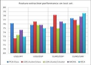
By nature of Forex, this is a variable depending on techniques as shown in Fig. 2 below. Table 3
the volatility and variance changes in the time series. represents the best results for each dataset using the
Our approach is to allow the classifier to predict the 3 classifiers over the test period.
sign of the 1) regardless of its value. The
motivation is that if 1) absolute value is
high; the features would have strong evidence for
correct classification and vice versa. And, for the
system to be profitable, it should classify high
changes accurately while it is not so important to
focus on small changes.
In this paper, three classifiers are used, namely; RBF,
MLP, and SVM. The percentage performance of each
classifier is calculated on the test data (252 days) by
simply looking at the % correct classification.
5.3 Percentage normalized profit (PNP):
We have developed a normalized profit criterion Fig. 2 Best Percentage Performance for Feature
which measures the success of the system Selection Techniques
predictions to follow the actual directions and
values of . Two classifiers may have the 5.4.2 Feature Extraction Results:
exact same classification performance but may give
significantly different profits since one of them is In this section we show the best percentage
predicting the important changes correctly and the performance resulted from the feature extraction
other is not. techniques for all the datasets as shown in Fig 3
Let the parameter P (t) be +1 if the prediction is below. Table 4 represents the best results for each
correct and P (t) is -2 if not. The reason is that, when dataset using the three classifiers over the test
a wrong decision is taken, the correct action is not period. For the feature extraction experiments using
taken, and further, since we have to take an action MCML, NCA and PCA, we used different number
each day, the wrong action is taken. Let the ideal of mapped features (5, 10, 15 and 20). In Table 4
profit represents the profit in case all the predicted we show the best results for each technique among
values were true. The normalized profit over a time the datasets.
duration T will be:
(1)
5.4 Experimental Results
Each of the feature selection and feature extraction
techniques discussed in section 4 produce a subset
of features. In all cases (except for the cluster-based
extraction), we have tried subsets ranging from 5 to
20 features. Each subset was used to train machine-
learning techniques, namely SVM, MLP and RBF.
We experimented with different parameters for each
classifier in order to reach the best performance on
each dataset.
Fig. 3 Best Percentage Performance for Feature
5.4.1 Feature Selection Results: Extraction Techniques
In this section we show the best percentage
performance resulted from the feature selection
ISBN: 978-1-61804-039-8 45Recent Researches in Applied Informatics and Remote Sensing
5.4.3 Prediction-based versus Ideal Profits: Table 5: Techniques Resulted in Best Performance and the
Highest Percentage Normalized Profit for Each Dataset
Fig. 4below shows: and Recognition
Dataset Best Technique PNP
rate
, this is drawn over T from 1 to 252 to see Bagging Trees
how the actual profit is progressing compared to the USD/JPY using (SVM) 77.8 61.9
ideal profit for the best profit resulted in each as classifier
technique. Table 5 represents the techniques with the Bagging Trees
best percentage performance over T from 1 to 252 USD/EGP using (MLP) 77.8 67
as classifier
with the best PNP over the same time period. Bagging Trees
EURO/EGP using (SVM) 78.6 67.7
as classifier
SVM – Based
EURO/SAR using (MLP) 79.8 60.8
as classifier
Fig. 4 Actual Profit vs. Ideal Profit for the best
technique
Table 3: Test Results(Percentage Performance)
Comparison using Machine Learning Techniques for Feature Selection Techniques
Dataset
USD/JPY USD/EGP EURO/EGP EURO/SAR
Selection technique
SVM MLP RBF SVM MLP RBF SVM MLP RBF SVM MLP RBF
Selection using SVM
77.4 75.4 75.8 72.6 72.2 72 78.2 77.8 77 77.8 79.8 77.8
Selection using bagging 77.8 73 73 74.6 77.8 75.8 78.6 76.6 77 78.2 77 77.8
tress
Table 4: Results(Percentage Performance)
Comparison using Machine Learning Techniques for Feature Extraction Techniques
Dataset
USD/JPY USD/EGP EURO/EGP EURO/SAR
Extraction technique
SVM MLP RBF SVM MLP RBF SVM MLP RBF SVM MLP RBF
PCA/Class
76.2 72.6 73 71.4 75.8 74.6 72.6 75 75.4 77 77.4 76.2
LDA(Cluster/ Class) 69.4 72.6 69 69.4 76.6 75 75 74.2 78.2 61.1 77 74.6
LDA(Cluster/ Cluster) 70.6 70.6 73.4 66.7 75.8 75.4 75 73 75 72.1 73.4 75.8
MCML 74.6 73 71.4 74.2 75 75.8 76.6 76.6 75.8 77.8 77.8 77.4
NCA 73 72.7 71.8 71 75 73.4 76.3 75.4 75 77 78.6 77
ISBN: 978-1-61804-039-8 46Recent Researches in Applied Informatics and Remote Sensing
6 Conclusion
[9] Dong-xiao Niu; Bing-en Kou; Yun-yun
In this paper we investigated Forex multiple time Zhang;
windows technical analysis and signal processing Coll. of Bus. & Adm., North China Electr. Power
features for predicting the high rate daily trend. The Univ., Beijing, China, ''Mid-long Term Load
prediction is posed as a binary classification problem Forecasting Using Hidden Markov Model'', pp 481 –
for which the system predicts whether the high rate is 483, 2009
going up or down. SVM-based and bagging trees [10] L Cao, Francis E H Tay, ''Financial Forecasting
feature selection methods as well as five feature Using Support Vector Machines'', Neural Computing
extraction techniques are all used to find best feature Applications (2001) vol. 10, Springer, pp: 184-192
subsets for the classification problem. Machine [11]Joarder Kamrwzaman' and Ruhul A Sarkeg,
learning classifiers (RBF, MLP and SVM) are all ''Forecasting of currency exchange rates using ANN:
trained using the many different feature subsets and A case study '', IEEE Int. Conf. Neural Networks 8
the results are shown and compared based on the Signal Processing, 2003
percentage classification performance. Also, a [12] Zhang, G.P.; Kline, D.M., ''Time-Series
percentage normalized profit function is invented Forecasting With Neural Networks'', Neural
which shows the ratio between the profit based on the Networks, IEEE, pp 1800 – 1814, 2007
predicted trends and that using ideal predictions. The [13] Woon-Seng Gad and Kah-Hwa Ng2,
results show that the proposed systems can be used ''Multivariate FOREX Forecasting using Artificial
for practical trading purposes. Neural Networks'', IEEE Xplore, 2010
[14]http://www.earningmoneyonlinearticles.com/inde
References x.php/trade-the-forex-market-without-any-challenges/
[15] Steven B. Achelis, Technical Analysis from A to
Z, McGraw-Hill, United States, 2nd Edition, 2001
[1] Deboeck, Trading on the Edge: Neural, Genetic
[16] http://forexsb.com/wiki/indicators/source/start
and F u q Systems for Chaotic Financial Markets,
[17]http://www.stockinvestingideas.com/technical-
New York Wiley, 1994.
analysis/technical-indicators.htm
[2] G. E. P. Box and G. M. Jenkins, Time Series
[18] Isabelle Guyon, Andr´e Elisseeff, '' An
Analysis: Forecasting and Control, Holden-Day, San
Introduction to Variable and Feature Selection'',
Francosco, CA
Journal of Machine Learning Research, pp 1157-
[3] H. B. Hwamg and H. T. Ang, “A Simple Neural
1182, 2003
Network for ARhlA@,q) Time Series,” OMEGA: lnt
[19] Alain Rakotomamonjy, '' Variable Selection
Journal of Management Science, vol. 29, pp 319-333,
Using SVM-based Criteria'', JMLR, 1357-1370, 2003
2002
[20] B. Ghattas, A. Ben Ishak, '' An Efficient Method
[4] G. Peter Zhang, ''Time series forecasting using a
for Variables Selection Using SVM-Based Criteria''.
hybrid ARIMA and neural network model'',
[21] http://www.dtreg.com/
Department of Management, Georgia State
[22] (MATLAB reference for the tree forest feature
University, January 2002
selection)
[5] Ching-Chun Wei, ''Using the Component GARCH
[23]http://homepage.tudelft.nl/19j49/Matlab_Toolbox
Modeling and Forecasting Method to Determine the
_for_Dimensionality_Reduction.html
Effect of Unexpected Exchange Rate Mean and
[24] Amir Globerson, Sam Roweis, '' Metric Learning
Volatility Spillover on Stock Markets'', International
by Collapsing Classes'', Advances in Neural
Research Journal of Finance and Economics, ©
Information Processing, 2006
EuroJournals Publishing, Inc. 2009
[25]http://en.wikipedia.org/wiki/Neighbourhood_com
[6] Dr. S S S Kumar, ''Forecasting Volatility –
ponents_analysis
Evidence from Indian Stock and Forex Markets'',
[26] P. Belhumeur, J. Hespanha, and D. Kriegman
2006
"Eigenfaces vs. Fisherfaces: Recognition Using Class
[7] Yu, J., (2002) “Forecasting Volatility in the New
Specific Linear Projection". IEEE PAMI, 1997.
Zealand Stock Market,” Applied Financial
Economics, 12: 193-202.
[8] Patrik Idvall, Conny Jonsson, '' Algorithmic
Trading
Hidden Markov Models on Foreign Exchange Data '',
Department of Mathematics, Link¨opings Universitet,
LiTH - MAT - EX - - 08 / 01 - - SE, 2008
ISBN: 978-1-61804-039-8 47You can also read