3-D Mobile Node Localization Using Constrained Volume Optimization Over Ad-Hoc Sensor Networks
←
→
Page content transcription
If your browser does not render page correctly, please read the page content below
3-D Mobile Node Localization Using Constrained
Volume Optimization Over Ad-Hoc Sensor Networks

                               Sudhir Kumar, Shriman Narayan Tiwari and Rajesh M. Hegde
                                                Department of Electrical Engineering
                                            Indian Institute of Technology Kanpur, India
                                            Email: {sudhirkr, shriman, rhegde}@iitk.ac.in

    Abstract—This paper proposes a three dimensional mobile          implementation of an algorithm which is simultaneously both
node localization and obstacle avoidance mechanism in ad-hoc         cost and computationally efficient and also has low memory
sensor networks (AHSN). The localization task is performed           requirement is a challenging task. The proposed algorithm
through constrained volume optimization. Obstacle avoidance          follows a distributed localization architecture over randomly
is achieved through weighted distribution method. Constrained        deployed sensor nodes. The applications of proposed algorithm
volume optimization is performed by minimizing the squared
                                                                     include vehicular tracking, security and surveillance.
location error and imposing the distance and boundary condi-
tions. Obstacle avoidance is achieved by choosing the angular           The notations used in this paper are described as follows.
direction which minimizes the cost function. The solution to the     The bold faced letters (either in lower or upper case) denote
constrained optimization problems ensures that the method is         one dimensional vector. (.)T represents transpose of a matrix
robust to change in environmental conditions and NLOS issues.
                                                                     and the L2 norm of the argument is represented by ||.||.
Additionally, the algorithm is scalable and follows a distributed
approach to localization. The performance of this method is             The rest of the paper is organized as follows. Section II
assessed by deploying nodes in both indoor and outdoor environ-      describes the 3-D mobile nodes localization using constrained
ments. Improved localization accuracy is noted when compared         volume optimization in detail. In Section III, performance
to conventional methods in terms of statistical location estimates
                                                                     evaluation and experimental results are discussed before con-
and Cramer-Rao lower bound localization error analysis.
                                                                     cluding the paper in Section IV.

                        I.   Introduction                                II.   3-D Mobile Node Localization using Constrained
                                                                                          Volume Optimization
    Three-dimensional localization in ad-hoc sensor networks
is one of the most challenging areas of research. A method               This Section presents the basic framework for mobile node
for three dimensional localization of sensor nodes has been          localization followed by a Section on distance estimation
described in [1]. Here, the localization accuracy is considerably    using multi-modal signals. Subsequently, the problem of 3-D
low as detailed in the performance evaluation Section. A             localization of mobile nodes is discussed. In the end, obstacle
distributed approach accelerates the localization process. The       avoidance for mobile node guidance is discussed.
computations are distributed to nodes and thus reduce the
computational delays, when compared to performance using             A. Basic framework for Mobile Node localization
a central system. A distributed approach of localization is
described in [2] using linear least square method. Following on          An undirected topology of the sensor networks is described
the similar lines a generic Monte-Carlo localization method for      by the tuple T = (N, E, W), where N, E and W represent the set
mobile node is discussed in [3]. [4] proposes a semi-definite        of sensor nodes, edges connecting pair of nodes and weights
algorithm for node localization and in [5] an accurate and           assigned to edges between each pair of nodes respectively.
cost effective algorithm for mobile nodes is discussed. During       Weights in this context refer to the received signal observations
measurements, often some of the observations suffer from non-        assuming one node is transmitting and other is receiving. The
line of sight (NLOS) communication issues. A few methods             weight is invariant in both direction i.e. {wi j = w ji } ∈ R.
which incorporate NLOS measurements have been discussed                  The location of sources are assumed to be known. Location
in [6–8].                                                            of the ith source is represented by (αi , βi , γi ), i ∈ S , where S is
                                                                     the set of source nodes. (xti , yit , zit ), i ∈ N denotes the location
    A localization algorithm which is computationally efficient
                                                                     of unknown ith mobile node at each instant t. The problem of
and has low energy consumption is crucial in building efficient
                                                                     localization is to find the location of these mobile nodes at each
wireless sensor network applications. This paper proposes a
                                                                     instant. To estimate the location of mobile nodes, distances
three dimensional mobile node localization technique using
                                                                     from each of the sources are computed. The distance between
constrained volume optimization. The proposed algorithm uses
                                                                     pair of nodes is estimated based on received signal strength
the signal observations as received signal vector to perform the
                                                                     [12, 13] and shown below.
localization task. There are existing methods based on received
signal strength (RSS) [9], time of difference of arrival (TDOA),                                                          λ
                                                                              Pt − Pr = 10ne log d − 10 log(Gt Gr ( )ne ) + χσ           (1)
time of arrival (TOA) [10], and direction of arrival (DOA) [11]                                                          4π
available in literature. It is widely accepted that the design and   where, Pt and Pr are the transmitted and received signal powers
978-1-4799-2361-8/14/$31.00 c 2014 IEEE                              in dB respectively. d, ne and χσ denote the distance between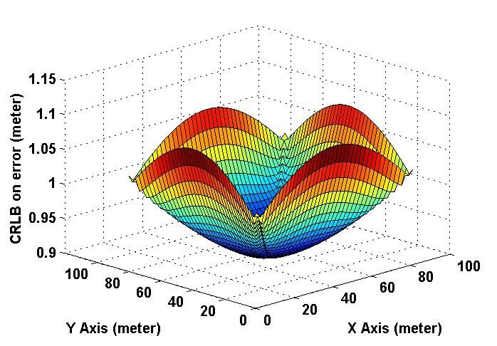
pair of nodes, path loss exponent and noise respectively. Gt , Gr   node can hear to. Since, the wireless channel is noisy, thus,
and λ are the transmitting antenna gain, receiving antenna gain     the intersection regions of all these spherical regions at any
and carrier wavelength respectively. In the following Section,      instant is not a point but a region as shown in Figure 1.
relationship between received signal and distance is established    Therefore, the estimated location of the mobile node is a point
experimentally for different modalities of signal.                  in the intersection region which minimizes the squared error
                                                                    as described in the following Section. It must be noted, that,
B. Development of Attenuation Models using Multiple Modal-          the experiments are conducted for mobile node localization
ities                                                               in a 3-dimensional space. However, it is equally applicable
                                                                    in a 2-dimensional scenario. This intersection region for 2-
    Experimental system is usually equipped with measuring          dimensional case is a planar region.
different signal modalities. This makes the localization process
easy and low cost. With the availability of different signal
modalities, localization can be performed using any one of
the signal modality. Experiments are conducted to collect data                                            R2
across different locations. The data is collected for received
signal observation, acoustic and light samples. Relationship                 R1
is established between received signal and distance between
source and node using Least-Squares approach. This method                                                                           Intersection
best fits the large number of measurements and also provides                                                                         Region
minimum Root Mean Squared Error (RMSE). The relations
may vary under different environmental conditions. In this
work, the experiments are conducted in Indian Institute of
Technology (IIT), Kanpur during autumn. The experiments are                               R3
conducted for the Crossbow motes. The relationship for the
received power with distance is represented as
                  Pr = −49.74 − 37.45 log(d)                  (2)   Fig. 1. Figure illustrating the formation of intersection region using overlap
                                                                    of circular regions
where, Pr represents the received power. The Euclidean dis-
tance between node and source is denoted by d. Now, the
experiment is repeated for the acoustic samples. At various         D. Constrained Volume Optimization Method Over an Am-
locations, acoustic samples are collected. Then relationship        biguous Region
between received acoustic samples with distance is captured
with the help of Equation 3.                                            The inter-nodal distance between a mobile node and a
                                                                    source, to which the node hears at instant t is computed using
                    Pr = 679 − 249.9 log(d)                   (3)   Equation 1. For distance calculation, relation between received
                                                                    signal observation and distance is established in Equation 5.
Similarly, for the case of light samples, the relationship is
                                                                    The objective of the proposed algorithm is to minimize the
represented as
                                                                    radial error, which is the squared difference of the actual
    Pr = −53.67 exp (0.4254d) + 808.7 exp (−0.02076d)         (4)   distance and the estimated distance from each of the sources
                                                                    [4]. Boundary conditions have been taken into account through
The fusion model using confidence-weighted averaging is             the first constraint. The second inequality in the constraints [6–
described in [14]. The fused signal model for received sig-         8] of Equation 6 takes care of the NLOS measurements. The
nal observation, acoustic and light can be obtained through         problem of node localization is then formulated as
Equation 5.
                  Pr = 45.94 − 35.38 log(d)              (5)                                    S
                                                                                                X
                                                                                  Minimize        |kXs − Xit k2 − d̃2s,i |2 W s,i
Node localization can be performed either using individual                                      s=1
signal modality or fused sensor data. Through experiments                       Subject to                                             (6)
it has been found that the localization accuracy improves by                                              i
using fused sensor data. It may be noted that Gt , Gr and                                      Xmin ≤ Xt ≤ Xmax
λ are captured as constants in Equations 2, 3, 4 and 5. In                                     kX s − Xit k ≤ d˜s,i ,  ∀s ∈ {S }
the following Section, 3-D localization of mobile nodes under                                    h                    i>
volume ambiguity is discussed.                                      where, Xmin           =        xmin ymin zmin          and Xmax =
                                                                    h                     i>
                                                                      xmax ymax zmax            are the minimum and maximum
C. 3-D Localization of Mobile Nodes under Volume Ambiguity          coordinate vectors      of  network
                                                                                       i>                 hin the giveni>reference frame.
                                                                    Xit = xti yit zit and X s = α s β s γ s are the vectors
                                                                          h
    The signals transmitted by a source are spread out omni-
directionally. Thus, if nth node receives a signal from sth         consisting of the coordinates of ith mobile node at instant t
source, which is located at a distance R from the node, then        and sth source node respectively. The estimated Euclidean
the node is likely to be inside a spherical region of radius        distance between ith mobile node and sth source node is
R with its center located at the position of the sth source.        represented by d̃2s,i . Here, d̃ s,i obtained is same as the distance,
The location of the node can be estimated by the intersection       d defined through Equation 1. W s,i represents the confidence
of these spherical regions from all the sources to which the        with which measurement are recorded at the node from each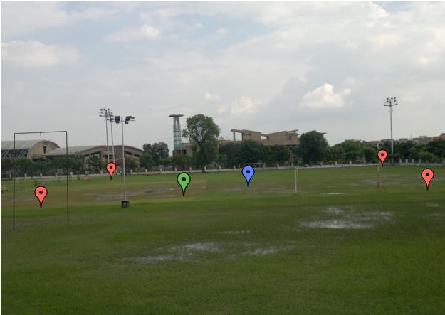
of the sources. A higher weight value signifies the reliability
of the received signal. For the experimental purpose, W s,i is
defined in Equation 7.

                      1 − exp(−Pr /Pt ) i f, Pr > 0.3Pt
                     (
           W s,i   =                                              (7)
                      0.26              otherwise
where, Pr and Pt are the received and transmitted power
respectively. Clearly, the problem formulated in Equation 6
is a non-convex problem. A solution to this problem becomes
a tedious task. So, to obtain a feasible solution, the problem
can be relaxed and can be reformulated as a convex problem.
   The function, f (Xit ) = |kXs − Xit k2 − d̃2s,i |2 is a non-convex    Fig. 2. Figure illustrating an angular region in 2-Dimensional plane with
                                                                         obstacle.
function. Let, Q be the region, where f (Xit ) is non-convex. So,
a convex relaxation to this function can be a function, g(Xit )
such that                                                                experiments. Experimental results on localization error have
                  g(Xit ) ≤ f (Xit ), ∀ Xti ∈ Q                    (8)   also been discussed.

    This convex relaxation is the tightest possible lower bound                            III.    Performance Evaluation
of this non-convex function [15]. This problem can be solved
by numerical techniques. Average localization improvement of                 In this Section, first Cramer-Rao bound analysis of local-
1.1m is obtained by using the constraints.                               ization error is presented. Subsequently, the results of mobile
                                                                         node localization for both indoor and outdoor environments
                                                                         are described.
E. Obstacle Avoidance Algorithm for Mobile Node Guidance
    This Section describes a mobile node guidance algorithm              A. Cramer-Rao Lower Bound (CRLB) Analysis
considering obstacle avoidance as described in [16]. The                    The CRLB of error variance of the proposed algorithm is
method uses a 2-dimensional Cartesian grid as the network                analysed through following expression [17].
model. The method employs a two step reduction process to
estimate the next direction of sensor. In the first step, a 2-                                              FRxx + FRyy
dimensional weight distribution is developed and is converted                                     σ2k ≥                2
                                                                                                                                              (9)
to a 1-dimensional angular weight distribution. Then, in the                                              FRxx FRyy − FRxy
next step from this 1-dimensional angular weight distribution            Equation 9 can also be represented as
the next direction of motion is selected. The two steps are                                           P          −2
described as follows.                                                                        1           i∈H(m) dk,i
                                                                                       σk = P
                                                                                         2
                                                                                                                                             (10)
    1) Computing Radial Weight Distribution for Optimal Path                                 b i∈H 0 (m) P M ( dk⊥i,   j di, j 2
                                                                                                                     2 2 )
                                                                                                                 j=i+1   dk,i dk, j
Selection : The 2-dimensional Cartesian grid is divided into
a number of small cells. The ultrasound sensors are used to              where, FRxx , FRxy , FRyy , b, dk⊥i, j and di, j are as described
derive the weights to each of these cells. Ultrasound signals are        in [17]. H(m) represents the set of M mobile nodes whose
transmitted exhaustively over the entire 2-dimensional plane.            location has been computed and H 0 (m) is the set of first M − 1
Based on the received signals on the receiver the weights                localized nodes. Similar CRLB expressions can be written as
of cells corresponding to the obstacle are incremented. From             in Equation 9 and 10 for each of the mobile nodes.
these weight values, the 2-dimensional weight distribution is
generated. The 2-dimensional region is then divided into n
                                                                         B. Localization Experiments in Indoor and Outdoor Scenarios
angular regions each of width α as shown in Figure 2. For
the experimental purpose n is taken to be six, this gives                    In this Section, performance of the algorithm is analysed
the value of α to be 60◦ . The weights lying in a particular             through extensive simulation and experiments. Subsequently,
region are summed and a 1-dimensional angular distribution is            real field deployment is done for both indoor and outdoor
formed. The horizontal axis of this 1-dimensional distribution           environments to validate the algorithm. The experiments are
corresponds to angular values (0◦ to 360◦ ), 0◦ taken to be the          conducted with the use of eight sources.
initial heading direction of the sensor. While the vertical axis
corresponds to the weights assigned to each of the angular                  1) Experimental Results in Indoor Environment: Indoor
values.                                                                  experiments have been conducted for a network dimension of
                                                                         20m ×20m ×5m. Crossbow motes, MTS310 sensor boards are
    Let G(θ) be the weight distribution as a function of angle           deployed both as sources and sensor node as shown in Figure
theta. From G(θ), choose that angle which minimizes the                  3. XM2110 IRIS board and MIB520 USB mote interface are
distance from the target and maximizes the alignment from                used as gateway to configure the network. Motes communicate
the target as described in [16].                                         with each other through IEEE 802.15.4 protocol.
    The following Section presents the results on mobile node               The average error and error variance of the proposed
localization for simulations as well as indoor and outdoor               algorithm for indoor experiments over time can be seen in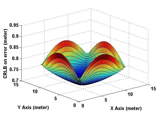
TABLE I. Table illustrating the average radial error for different experimental conditions over time for communication range (R) = 55% of network
dimension
T = 10 T = 20 T = 30 T = 40 T = 50 T = 60 T = 70 T = 80 T = 90 T = 100
Simulation 6.06 5.98 5.97 5.97 5.95 5.96 5.94 5.93 5.93 5.87
Outdoor Experiment 6.56 6.47 6.45 6.48 6.55 6.55 6.50 6.53 6.57 6.55
Indoor Experiment 1.82 1.70 1.70 1.72 1.78 1.71 1.69 1.70 1.68 1.69
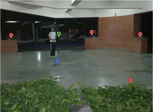
Fig. 3. Figure illustrating the indoor experimental deployment: four sources
(Crossbow motes MTS310) are shown shown in red, mobile mote in green
and gateway (XM2110 IRIS board and MIB520 USB mote interface) in blue Fig. 5. Figure illustrating the CRLB for indoor deployment in 2-dimensions
Table I. Low variance in estimation error over time signifies the
robustness of the proposed algorithm. The minimum variance
of error obtained from the CRLB [17, 18] is 0.72m, as shown
in Figure 5, which indicates significantly better performance.
2) Experimental Results in Outdoor Environment: Outdoor
experiments are conducted by deploying the sensor nodes and
source in a network of 100m × 100m × 5m. Eight National
Instruments (NI) WSN - 3212 and 3202 nodes are deployed
as source nodes in the network as shown in Figure 4. NI 9792,
gateway communicates to the nodes using IEEE 802.15.4
protocol.
Fig. 6. Figure illustrating the CRLB for outdoor deployment in 2-dimensions
I. Thus, the low variance in localization error over time for
simulations, indoor and outdoor experiments show efficient
performance of the proposed algorithm. The following Sec-
tion presents the localization error analysis of the proposed
algorithm when compared with other algorithms.
C. Localization Error Analysis
Average radial error is chosen as a measure of performance
Fig. 4. Figure illustrating the outdoor experimental deployment: four sources
(NI 3202 WSN node) are shown in red, mobile node (NI 3212 WSN node) analysis. Average radial error is defined as the absolute dis-
in green and gateway (NI 9792) in blue tance between actual and estimated node location at an instant
averaged over large number of observations. Localization error
analysis is performed by computing the effect of change
The average error and average error variance of the pro- of time duration on radial error. The effect of change of
posed algorithm for outdoor experiment over time can be seen communication range on average localization error is also
from Table I. A very less variation in the estimation error is observed. Experiments are conducted using eight sources and
observed, this indicates the robustness of proposed algorithm one mobile node. However, the localization task can be easily
over time. The minimum variance of the error is found to be performed for multiple nodes and sources.
0.92m as shown in Figure 6 [17, 18], which shows the efficient
The sources are placed symmetrically on the boundary of
performance of the proposed method.
the rectangular deployment region whereas, the node is mobile
The result for the simulated data are also shown in Table in nature. The node can traverse at any speed within a speed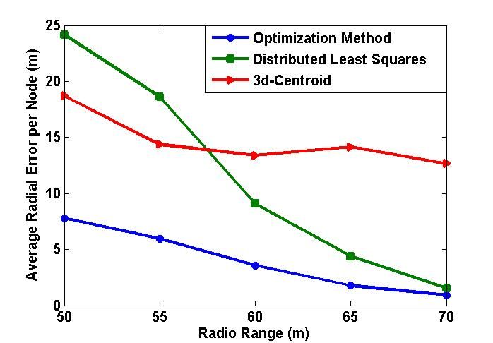
range of 0 to 10 m/s.                                                          the impact of wireless channel and variation of received signal
                                                                               observation with time and due to environmental conditions
    1) Average Localization Error over Time: The proposed                      with the help of the volume constraints. The application of
algorithm and other two algorithms, 3D-Centroid algorithm                      the algorithm to both LOS and NLOS communications makes
[1] and distributed least square algorithm [2] for 3-dimension                 it robust. The proposed algorithm performs consistently well
are compared by varying time duration of localization process                  irrespective of the variation in the localization duration and
as shown in Figure 7. The effect of varying time duration is                   radio communication range. The focus of future work is
observed on average radial error. The proposed optimization                    on developing a three dimensional localization algorithm in
algorithm outperforms the two algorithms [1] and [2].                          mobile sensor networks using mobile nodes and anchors.

                                                                                                     Acknowledgment
                                                                                  This work was supported in part by Indian Space Research
                                                                               Organisation (ISRO).

                                                                                                         References
                                                                                [1] H. Chen, P. Huang, M. Martins, H. C. So, and
                                                                                    K. Sezaki, “Novel centroid localization algorithm for
                                                                                    three-dimensional wireless sensor networks,” in Wire-
                                                                                    less Communications, Networking and Mobile Comput-
                                                                                    ing, 2008. WiCOM’08. 4th International Conference on.
                                                                                    IEEE, 2008, pp. 1–4.
                                                                                [2] F. Reichenbach, A. Born, D. Timmermann, and R. Bill,
Fig. 7. Figure illustrating average localization error over time. Communica-
                                                                                    “A distributed linear least squares method for precise
tion Range (R) = 55m                                                                localization with low complexity in wireless sensor net-
                                                                                    works,” in Distributed Computing in Sensor Systems.
    2) Effect of Varying Radio Communication Range: To                              Springer, 2006, pp. 514–528.
evaluate the performance of the proposed algorithm, Figure                      [3] H. Xu, J. Luo, and M. Luo, “Mobile node localization al-
8 shows the variation of average localization error with the                        gorithm in wireless sensor networks for intelligent trans-
change in radio communication range. The proposed opti-                             portation systems,” in Distributed Computing and Appli-
mization algorithm has better performance for all values of                         cations to Business Engineering and Science (DCABES),
communication range, as seen from Figure 8. A node can hear                         2010 Ninth International Symposium on. IEEE, 2010,
many sources, if communication range of source is larger. This                      pp. 491–494.
helps in decreasing the location uncertainty of the node as                     [4] P. Biswas and Y. Ye, “Semidefinite programming for ad
seen from Figure 8. For communication range of 70m, average                         hoc wireless sensor network localization,” in Proceed-
radial error comes below 1m in the given network.                                   ings of the 3rd international symposium on Information
                                                                                    processing in sensor networks. ACM, 2004, pp. 46–54.
                                                                                [5] S. Alikhani, M. St-Hilaire, and T. Kunz, “icca-map: a
                                                                                    new mobile node localization algorithm,” in Wireless and
                                                                                    Mobile Computing, Networking and Communications,
                                                                                    2009. WIMOB 2009. IEEE International Conference on.
                                                                                    IEEE, 2009, pp. 382–387.
                                                                                [6] S. Venkatesh and R. M. Buehrer, “Nlos mitigation us-
                                                                                    ing linear programming in ultrawideband location-aware
                                                                                    networks,” Vehicular Technology, IEEE Transactions on,
                                                                                    vol. 56, no. 5, pp. 3182–3198, 2007.
                                                                                [7] E. Larsson, “Cramer-rao bound analysis of distributed po-
                                                                                    sitioning in sensor networks,” Signal Processing Letters,
                                                                                    IEEE, vol. 11, no. 3, pp. 334–337, 2004.
                                                                                [8] I. Guvenc and C.-C. Chong, “A survey on toa based
                                                                                    wireless localization and nlos mitigation techniques,”
Fig. 8. Figure illustrating the effect of change of radio communication on          Communications Surveys Tutorials, IEEE, vol. 11, no. 3,
average localization error                                                          pp. 107–124, 2009.
                                                                                [9] E. Goldoni, A. Savioli, M. Risi, and P. Gamba, “Experi-
                           IV.    Conclusion                                        mental analysis of rssi-based indoor localization with ieee
                                                                                    802.15. 4,” in Wireless Conference (EW), 2010 European.
     In this paper, a three dimensional localization algorithm                      IEEE, 2010, pp. 71–77.
for mobile nodes along with obstacle avoidance mechanism                       [10] S. K. Meghani, M. Asif, and S. Amir, “Localization of
is proposed. The performance of the algorithm is analysed by                        wsn node based on time of arrival using ultra wide band
varying the communication range. Cramer-Rao lower bound                             spectrum,” in Wireless and Microwave Technology Con-
analysis is also performed. Performance is evaluated for both                       ference (WAMICON), 2012 IEEE 13th Annual. IEEE,
indoor and outdoor deployments. The algorithm accounts for                          2012, pp. 1–4.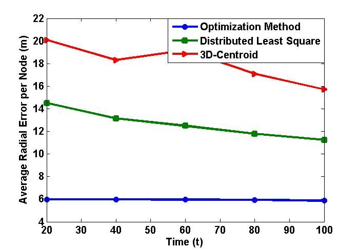
[11] F.-K. Chan and C.-Y. Wen, “Adaptive aoa/toa localization     [15] [Online].    Available:    http://www.winlab.rutgers.edu/
     using fuzzy particle filter for mobile wsns,” in Vehicular        ∼crose/322 html/convexity2.pdf
     Technology Conference (VTC Spring), 2011 IEEE 73rd.          [16] J. Borenstein and Y. Koren, “The vector field histogram-
     IEEE, 2011, pp. 1–5.                                              fast obstacle avoidance for mobile robots,” Robotics and
[12] T. S. Rappaport et al., Wireless communications: princi-          Automation, IEEE Transactions on, vol. 7, no. 3, pp. 278–
     ples and practice. Prentice Hall PTR New Jersey, 1996,            288, 1991.
     vol. 2.                                                      [17] N. Patwari, A. O. Hero III, M. Perkins, N. S. Correal,
[13] M. Bertinato, G. Ortolan, F. Maran, R. Marcon, A. Mar-            and R. J. O’dea, “Relative location estimation in wireless
     cassa, F. Zanella, M. Zambotto, L. Schenato, and                  sensor networks,” Signal Processing, IEEE Transactions
     A. Cenedese, “Rf localization and tracking of mobile              on, vol. 51, no. 8, pp. 2137–2148, 2003.
     nodes in wireless sensors networks: Architectures, algo-     [18] S. Kumar, V. Sharan, and R. M. Hegde, “Energy efficient
     rithms and experiments,” 2008.                                    optimal Node-Source localization using mobile beacon
[14] A. Schörgendorfer and W. Elmenreich, “Extended                   in Ad-Hoc sensor networks,” in Globecom 2013 - Ad
     confidence-weighted averaging in sensor fusion,” in Pro-          Hoc and Sensor Networking Symposium (GC13 AHSN),
     ceedings of the Junior Scientist Conference JSC, vol. 6,          Atlanta, USA, Dec. 2013, pp. 509–514.
     2006, pp. 67–68.
You can also read