The "Astropeiler Stockert Story" Part 7: Pulsar Observations
←
→
Page content transcription
If your browser does not render page correctly, please read the page content below
The "Astropeiler Stockert Story"

Part 7: Pulsar Observations
Wolfgang Herrmann

1. Introduction
This is the seventh and final part of a series of articles to introduce and describe the
"Astropeiler Stockert", a radio observatory located on the Stockert Mountain in
Germany. This observatory comprises a 25 m dish, a 10 m dish and some other
smaller instruments. It is maintained and operated by a group of amateurs and is as
of today the world's most capable radio observatory in the hands of amateurs.

In this series of articles I wish to describe the setup, the instrumentation and the
observational results achieved.
This eighth part of the series will deal with observation of pulsars.

2. Pulsars
Pulsars are one of the most interesting objects for radio astronomy. For amateurs,
they are considered somewhat as the "holy grail" of observational achievements.
This is due to the fact that pulsar signals are quite weak and it takes special effort to
observe these faint signals.

The basic mechanism of pulsars is reasonably understood these days. However, the
details of the pulsar emission is still not fully explained by theoretical models yet.
Therefore, pulsars are an area of intensive research even decades after their first
detection. It all started with a serendipitous discovery by Jocelyn Bell in 1967,
published in 1968 [1]. Since then, more than 2500 pulsars have been detected with
periods ranging from a couple seconds down to the millisecond range. The most
comprehensive data base of pulsars is maintained by the Commonwealth Scientific
and Research Organization (CSIRO) and can be found at [2].
There is a wealth of information on the nature of pulsars and their mechanisms.
Therefore I would like to refrain from trying to go in depth here, but rather refer to
some available online resources such as [3]. This list of resources has been compiled
by Steve Olney on his website [4] which deals with amateur observation of pulsars.

The ambitious reader with a special interest in this matter is recommended to refer to
the book "Handbook of Pulsar Astronomy" by D. Lorimer and M. Kramer [5].

As a summary of the main characteristics pulsars I would like to highlight just a few
facts:
•   Pulsars are considered to be objects which consist primarily of highly densely
    packed neutrons with a mass of up to 1.4 solar masses and a diameter of 10-
    20 km.
•   Pulsars are considered to be formed as a leftover after a supernova
    explosion. While most of the matter is carried away in the explosion, a certain
    part is reformed into an object which is extremely compacted by its own
    gravitational force.
•   Due to the conservation of the angular momentum of the material of the
    progenitor star, pulsars rotate very fast as they have become so small.
•   Also, the magnetic field is intensified as a result of the small diameter.
    Therefore, pulsars form a extremely strong magnetic dipole.
•   The rotational axis and the axis of the magnetic field are (typically) inclined
    away from each other.
•   As the magnetic field rotates it passes through charged particles surrounding
    the pulsar, electromagnetic radiation is generated which propagates along the
    axis of the magnetic field.
•   The radiation is broadband, starting in the 10's of MHz and extending into the
    microwave range. Typically, the largest intensity is in the UHF range,
    dropping off with higher frequencies.
•   If the rotating beam of radiation happens to pass the earth on each rotation, a
    brief pulse is received, hence the name "pulsar".

                         Figure 1: Principle of a pulsar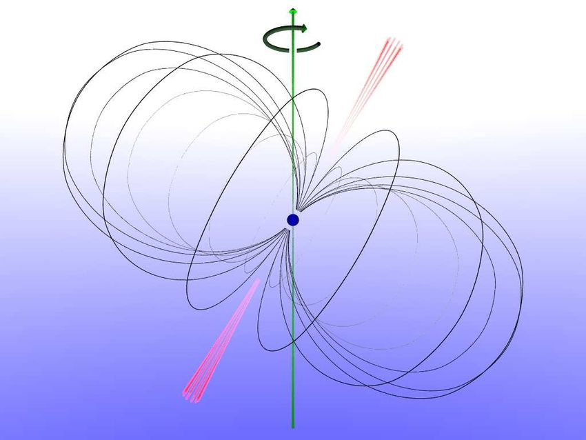
3. Propagation of pulsar radiation through the interstellar medium

3.1. Dispersion

The radiation from a pulsar is influenced by the characteristics of the interstellar
medium between the pulsar and the observer. This has an impact on the
observational methods and the signal processing required.

The most important effect is dispersion. As the interstellar medium is a thin plasma
(electrons and protons are present, albeit in very low density) the propagation speed
becomes frequency dependent. Lower frequencies will be delayed more than higher
frequencies as depicted in fig. 2.

                                                                                   Increasing
                                                                                   frequency
                                                                                        f1
                                                                                        f2
                                                                                        f3
                                                                                        f4

                                                                           Time
                   Arrival time differs depending on frequency

                                         Figure 2: Dispersion

As a result, the signal from a pulsar will be smeared, becoming wider and possibly
even undetectable if this effect is not accounted for. The time difference (in
millisceonds) between the arrival times t1 and t2 at two frequencies is f1 and f2 given
by:

t2 - t1 = 4.15 DM [( f1 )-2 - ( f2 -2]                                       (1)

where f1 and f2 are the frequencies in GHz and DM is a value specific to the pulsar.
DM stands for "dispersion measure" and is the product of the electron density (on the
path between the pulsar and the observer) and the distance in parsec.
Therefore, measuring the dispersion allows to determine the distance to a pulsar if
the electron density is known or vice versa.
3.2. Scintillation A second effect caused by the interstellar matter is scintillation. It is similar to the twinkling of stars in the optical regime. The twinkling is caused by fluctuations of the atmosphere. For pulsars, however, the cause is fluctuations of the interstellar matter which affect the various propagation paths of the pulsar radiation. This causes sometimes negative and sometimes positive interference between the various paths. This is the reason for fluctuations of the pulsar signal. In case of positive interference the signal can be enhanced significantly whereas in time of negative interference the signal may be very low. Variations up to a factor of 10 can be observed in a number of pulsars. The time scale of these fluctuations vary also substantially; from sub-second to hours depending on the pulsar. 4. Observational Methods 4.1. Signal acquisition We observe the pulsars with 97 MHz of bandwidth, centred at 1380 MHz. The signal is down converted to an IF of centred at 150 MHz. Both linear polarizations are received. The signal is then fed into a fast Fourier transform spectrometer. This spectrometer has been described briefly in the second part of this series [6]. For pulsar observations, this spectrometer is used in PFFTS (Pulsar Fast Fourier Transform Spectrometer) mode. Details about this mode can be found in section 3.2 of [7]. In this mode, the spectral resolution is about 585 kHz. Depending on the setting, the time resolution can be as high as 54 µsec. In most cases, a more moderate resolution of 218 µsec is used to reduce the amount of data. The data delivered from the spectrometer (168 spectral channels for each cycle) amounts to about 2 to 12 MByte/s depending on the time resolution chosen. The data is recorded in a file. This data represents the spectrum for each time slot. 4.2. Signal processing This raw data is processed in essentially two steps: The first step is the so called de-dispersion to account for the effect described in 3.1. In this process, each spectral channel is adjusted in time to compensate for the dispersion. Since we are observing known pulsars, the dispersion measure is known and can be used to do the proper de-dispersion. The de-dispersion process is depicted in fig. 3.
(De-Dispersion)

                                                                                         f1
                                                                                         f2
                                                                                         f3
                                                                                         f4

                            Figure 3: De-dispersion process

In this way, all spectral channels are combined into one signal which represents the
power received over time. This signal is called a "time-series".

The second step is to further process the time series.
As pulsar signals are quite weak, typically single pulses cannot be seen in the time
series data. Many pulses have to be averaged in order to get a detectable signal.
This averaging is performed by a process called "folding". The time series is cut into
chunks with a length of the pulsar period each. Each of these chunks is then added
in order to provide an average. In this way, the SNR is greatly enhanced.
Again, as the period of known pulsars can be taken from the literature, this known
period can be used as a parameter in the folding process. The folding process is
depicted below in fig. 4.
+ +
Figure 4: Folding process
4.3. Timing corrections
There are several caveats with the period taken from the literature, though. While
pulsars have a very stable period, there is still some decline in rotation called "spin
down". This is due to the energy lost by the pulsar over time by the emitted radiation.
Therefore, if the period was measured some time ago, this spin down has to be taken
into account.
An even more important effect is the motion of the observer with respect to the
pulsar. As the earth rotates around the sun, the moon rotates around the earth and
"wobbles" the earth, the rotation of the earth itself and other factors the apparent
period of the pulsar changes due to the Doppler effect. Therefore, pulsar periods are
given with respect to the solar system barycentre in the literature. For any
observation, the observable period (called topocentric period) has to be calculated
from the barycentric period and the spindown has to be taken into account to get the
proper period to be used for folding.
4.4. Timing requirements
Folding a long time series from a fast pulsar requires a high stability and accuracy of
the timing. Consider a on hour observation of a millisecond pulsar: You want keep
the phase for folding to within a few percent of the pulsar period over the observation
period. For our fastest pulsar and 5% allowable phase shift, this would be 75 µsecover one hour, which means a clock accuracy of ~ 2*10-8. We therefore use a rubidium standard for clocking all our devices. 4.5. RFI mitigation Due to low level of pulsar signals, interference from terrestrial radio sources becomes a very important factor for signal degradation. Therefore, we typically use RFI mitigation techniques where affected spectral channels are removed and spikes (such as from radar interference) are clipped. 4.6. Software used All the signal processing and analysis is done by software from the professional radio astronomy community. It is a great advantage that these sophisticated tools are publicly available. Initially we have used the SIGPROC package [8] by Duncan Lorimer and may other contributors. More recently we have been using PRESTO [9] by Scott Ransom who also had contributions from various people. Timing calculations are done using TEMPO [10] and/or TEMPO2 [11], [12]. Minor additions were made to all these packages in order to introduce an additional observatory code so that our observatory and its location is properly recognized and correctly reflected in the timing calculations. 4.7. Source of pulsar ephemeris and flux data The CSIRO data base mentioned above, called the ATNF pulsar catalogue, was used to select suitable pulsars for observation attempts. All data used in post processing our observations was taken from this catalogue. 5. Observation Results So far we have observed 112 pulsars, ranging in period from 3.7 sec (B0525+21) down to 1.5 msec (B1937+21). At the observing frequency, the flux density of the strongest pulsar (B0329+54) is 203 mJansky 1). The weakest pulsar observed so far (J0621+0336) has a flux density of 1 mJansky. The dispersion measure ranged from 2.96 (B0950+08) to 622 (B1815-14). The integration time for the observations varied between a few and 100 minutes. Below is a list of all pulsars observed to date, giving the name, the period, the dispersion measure and the flux as provided by the ATNF data base (Table 1).
NAME       P0       DM         S1400       NAME        P0       DM         S1400
             (s)   (cm^-3 pc)    (mJy)                   (s)   (cm^-3 pc)    (mJy)
B0011+47     1.241       30.85       3.0   B1749-28      0.563      50.37       18.0
B0031-07     0.943       11.38      11.0   B1754-24      0.234    179.454        3.9
B0136+57     0.272       73.75       4.6   B1804-08      0.164     112.38       15.0
B0138+59     1.222     34.797        4.5   B1815-14      0.291        622        7.1
B0144+59     0.196       40.11       2.1   B1818-04      0.598      84.38        8.0
J0215+6218   0.549          84       3.7   B1821-19      0.189    224.648        4,9
J0248+6021   0.217         370      13.7   B1822-09      0.769      19.46       10.8
B0301+19     1.388     15.737        3.0   B1826-17      0.307     217.11        7.7
B0329+54     0.715       26.83     203.0   B1829-08      0.647    300.869        2.1
B0353+52     0.197     103.71        1.9   B1831-03      0.687    234.538        2.8
B0355+54     0.156       57.03      22.9   B1831-04      0.290     79.308        5.0
B0402+61     0.595        65.3       2.8   B1834-10      0.563     316.98        3.7
B0450+55     0.341     14.602       12.9   B1839+56      1.653     26.698        4.0
B0450-18     0.549       39.93       5.3   B1838-04      0.186     325.49        2.6
B0458+46     0.639       42.19       2.5   J1840-0809    0.956      349.8        2.3
B0523+11     0.354       79.34       1.6   B1844-04      0.598    141.979        4.3
B0525+21     3.746       50.94       9.0   B1844+00      0.461     345.54        8.6
B0531+21     0.034     56.791       14.4   B1845-01      0.659     159.53        8.6
J0538+2817   0.143       39.57       1.9   B1857-26      0.612     37.994       13.0
B0540+23     0.246     77.698        8.9   B1859+03      0.655     402.08        4,2
B0559-05     0.396     80.538        2.5   B1900+01      0.729    245.167        5.5
B0609+37     0.298       27.14       4.0   J1901-0906    1.782     72.677        3.1
B0611+22     0.335       96.91       2.1   B1911-04      0.826     89.385        4.4
J0621+0336   0.270       72.59       1.0   B1915+13      0.195     94.494        1.9
B0626+24     0.477     84.195        3.2   B1919+21      1.337      12.46        6.0
B0628-28     1.244       34.36      23.4   B1929+10      0.227        3.18      36.0
J0646+0905   1.388     15.737        3.6   B1933+16      0.359     158.52       42.0
B0656+14     0.384     13.997        3.7   B1937+21     0.0015      71.04       13.8
B0740-28     0.167       73.77      23.0   B1944+17      0.441        16.3      10.0
B0809+74     1.292        6.12      10.0   B1946+35      0.717     129.07        8.3
B0818-13     1.238       40.94       7.0   B1952+29      0.427      7.932        8.0
B0820+02     0.865       23.73       1.5   B1953+50      0.519     31.974        4.0
B0823+26     0.531     19.463       10.0   B2000+40     0.9051    131.334        4.9
B0834+06     1.273       12.85       4.0   B2011+38      0.230     238.22        6.4
B0906-17     0.402     15.888        3.2   B2016+28      0.558      14.17       30.0
B0919+06     0.431     27.309        4.2   B2020+28      0.343      24.64       38.0
B0950+08     0.253        2.96      84.0   B2021+51      0.529      22.65       27.0
J1022+1001   0.016    10.2521        6.1   B2022+50      0.373     33.021        2.2
B1039-19     1.386     33.777        4.0   B2044+15      1.138      39.84        1.7
B1112+50     1.656       9.195       3.0   B2045-16      1.962      11.46       13.0
B1133+16     1.188       4.848      32.0   B2106+44      0.415    139.827        5.4
B1237+25     1.382       9.296      10.0   B2111+46      1.015     141.26       19.0
B1508+55     0.740       19.61       8.0   J2145-0750    0.016     8.9977        8.9
J1518+4904   0.041   11.61139        4.0   B2148+52      0.332     148.93        2.0
B1540-06     0.709        18.4       2.0   B2148+63      0.380        128        2.9
B1541+09     0.748       35.24       5,9   B2154+40      1.525      70.86       17.0
B1604-00     0.422       10.68       5.0   B2217+47      0.538     43.519        3.0
B1642-03     0.388       35.73      21.0   B2224+65      0.683      36.08        2.0
B1700-32     1.212    110.306        7.6   B2255+58      0.368     151.08        9.2
B1702-19     0.299     22.907        8.0   B2303+30      1.576     49.544        2.2
J1713+0747   0.005    15.9915        7.4   B2310+42      0.349        17.3      14.6
B1718-35     0.280         496      11.0   B2319+60      2.256      94.59       12.0
B1737+13     0.803        32.7       3.9   B2324+60      0.234    122.613        4.4
B1737-30     0.606         153       6.4   B2327-20      1.644      8.458        3.0
J1740+1000   0.154       23.85       9,2   J2346-0609    1.181        22.5       2.0
B1742-30     0.367        88.8      14.1   B2351+61      0.945     94.662        5.0
                        Table 1: List of observed pulsars
5.1. Some specific pulsars
B0329+54
The strongest pulsar in the northern hemisphere is B0329+54 with a period of
714 ms. Not only is it the strongest pulsar, it also has some interesting features:
First, it is not just a simple pulse but the shows a structure with a pre- and a post-
pulse:
Figure 5: Observed pulse profile of B0329+54 (intensity in arbitrary units)
The horizontal scale is the rotation phase of the pulsar in degrees,
i.e. it represents one rotation of the pulsar
Due to its strength there is an excellent signal to noise ratio for this observation.
However, the strength varies substantially over timescales of typically 30 min or so.
This is the effect of scintillation which is quite prominent with this pulsar.
This is demonstrated in fig. 6. Here the signal intensity observed from this pulsar is
plotted over a few hours. It shows substantial variations which is typical for a pulsar
with strong scintillation.120
100
80
60
40
20
0
14:00 14:30 15:00 15:30 16:00 16:30 17:00 17:30 18:00 18:30 19:00 19:30
Figure 6: Intensity variations of B0329+54 due to scintillation
B2020+28
This pulsar has a nice double peak as shown below in fig. 7. The period is 343 ms.
Figure 7: Observed pulse profile of B2020+28 (intensity in arbitrary units)B1749-28
A real "classical" example is this pulsar shown in fig. 8: A single pulse, a typical
period of 563 ms and a "mid range" dispersion measure of 50.4.
Figure 8: Observed pulse profile of B1749-28 (intensity in arbitrary units)
B1937+21
This is the fastest pulsar from our collection. It is also the second fastest pulsar
known with a period of only 1.558 ms, beaten only by J1748-2446ad which has a
period of 1.396 ms.
At this short period we are getting to the limits of our time resolution. Therefore, the
resolution of the pulse shape of this pulsar is limited as can be seen in fig. 9.
Nevertheless it is resolved that this pulsar has a main pulse and a second pulse (the
"inter-pulse") separated by almost 180° in phase from the main pulse.Figure 9: Observed pulse profile of B1937+21 (intensity in arbitrary units) 6. Special effects in pulsars Besides the effects due to the interstellar matter as described in section 3., there are other interesting effects which are intrinsic to the pulsar. These will be described in this section. 6.1. Mode changing The pulse shape and intensity of a pulsar varies from pulse to pulse. However, after averaging a number of pulses (in the order of a few tens to 100 pulses) there will be a very stable profile which is characteristic to this pulsar. This is valid for most of the pulsars. There are a few, however, which change their pulse profile from time to time very abruptly. Such a change takes place within seconds. The time when such a change happens cannot be predicted, there is no recognizable pattern.
A very prominent example of such a mode changing pulsar is B0329+54 which has
been described above. The profile as shown in fig. 5 can change abruptly and then
look like as observed in fig. 10:

                    B0329+54 ; Period 0.714 sec ; abnormal mode

                Figure 10: Pulse profile of B0329+54 in abnormal mode
                      Insert shows normal mode for comparison

This mode is called "abnormal" mode. About 20% of the time the pulsar is in this
abnormal mode where the intensity of the pre- and post pulse are inverted compared
to the normal mode.

6.2. Giant pulses

The intensity of a pulsar will typically vary from pulse to pulse. Variations of up to a
factor of 10 are not uncommon. However, there are some pulsars where there are
very strong pulses in between the normal pulses, exceeding this ratio by far. These
very high pulse are called "giant pulses".

The most prominent example for such a behaviour is the Crab pulsar which I will
present in this section. This also gives the opportunity to present the usage of the
PRESTO package.
Figure 11: PRESTO analysis of a Crab pulsar observation The graphical output from PRESTO (fig 11) provides quite a bit of information: In the upper left corner there is the profile of the pulsar. It is shown twice simply for the purpose that no matter how the phase of the observation is, always a full profile is shown. The profile of the Crab pulsar has an interpulse which can be seen in the plot (just like the B1937+21 shown in fig. 9). Below the profile there is a grey scale picture showing how the signal has been developing over the observation time, together with a graph of the increase of the SNR. The other grey scale image in the middle shows the pulsar intensity as a function of frequency. As mentioned, we have 97 MHz of bandwidth which are split in 84 sub- bands in this analysis. The graph below this grey scale plot shows the SNR as a function of the dispersion measure. Obviously there is a clear maximum at the DM of the Crab pulsar. The three plots at the right of the output show the SNR as a function of period and the first derivative of the period (the spin down). For a short observation like this (about 26 minutes) one cannot expect to get a value for the spin down. It is just determined to be 0 (+/- 3.7*10-11 s/s2).
PRESTO can do a search for single pulses set which are high enough emerge from
the noise in the data.
The result of this analysis is shown the output below (fig. 12)

             Figure 12: Single pulse analysis of a Crab pulsar observation

The first three graphs show the number of detected single pulses and their dispersion
measure. It can clearly be seen that there are numerous single pulses with exactly
the DM of the Crab pulsar. The most prominent single pulse has a SNR of about 300
with the right DM.
The lower graph shows the occurrence of single pulses over the observation period.
The circle diameters are a measure of the intensity and this also demonstrates that
there are strong pulses at the DM of the crab pulsar. In contrast to this, there is a
single pulse at about 800 s which shows no DM dependency and therefore is a RFI
pulse.
Another demonstration of the giant pulses from the Crab pulsar is shown below in fig.
13:
30000000000
25000000000
Average x 100
Single Pulse
20000000000
15000000000
10000000000
5000000000
0
0 50 100 150 200 250 300
-5000000000
Figure 13: Single pulse analysis of a Crab pulsar observation
Vertical scale: arbitrary intensity
Horizontal scale: Pulsar period divided into 256 time bins
Here the average signal (red) is shown in comparison with the raw, non averaged
data (blue). The average signal has been increased by a factor of 100 over the non
averaged data. The non averaged data has been cut off below a certain threshold for
clarity of the plot.
One can see, that the largest pulse is about 800 times higher than the average pulse.
Also, there is a giant pulse at the time of the interpulse.
This data has been evaluated with respect to the number of pulses observed at a
certain ratio of the giant pulse intensity to the average pulse intensity.
This relation follows a log-normal distribution (fig 14):100
Cumulative Number of Pulses
10
1
10 100 1000
Peak Flux / Average Peak Flux
Figure 14: Log normal distribution of giant pulses
Giant pulses were also observed from B1133+16 with pulses up to 35 times the
average pulse intensity; and B0950+08 with pulses up to 30 times the average pulse
intensity.
Both pulsars are known from the literature to produce giant pulses.
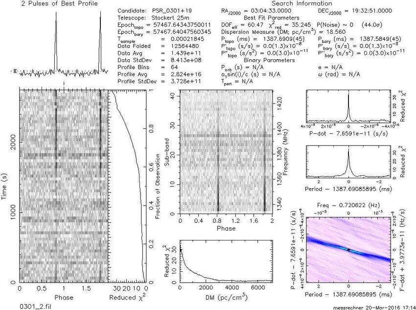
6.3. Nulling
Some pulsars exhibit the phenomenon of "nulling". This is when a pulsar abruptly
stops sending pulses for a brief period and resumes pulses shortly thereafter.
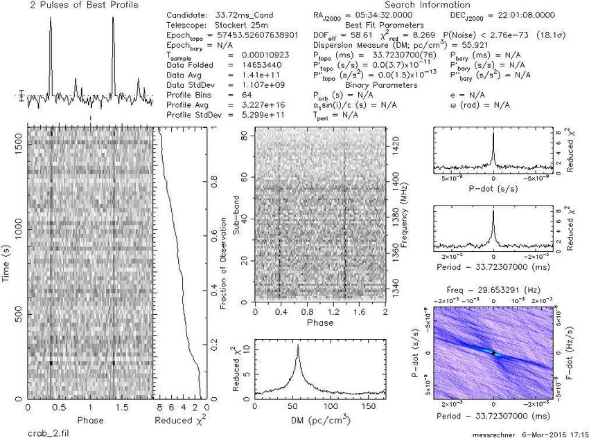
An example of such a behaviour was recorded during a ~45 minutes observation of
the pulsar B0301+19 as shown below in fig. 15:Figure 15: Nulling of PSR B0301+19
First one notices that this pulsar shows strong scintillation over a long time period as
demonstrated by the gradual increase of the intensity. However, at about 2500
seconds into the observation, there are two sudden interruptions where no signal is
observed and the cumulated SNR remains constant. For better clarity, an excerpt of
the plot is shown below in fig. 16. This is the typical pattern of nulling.
Figure 16: Detail view of nulling at ~ 2500 sec7. P-Pdot Diagram
One way of representing the "zoo" of pulsars is the so-called P-Pdot diagram. P
stands for the period and Pdot for the first derivative of the period, i.e. the spin-down
rate. Below in fig. 17 such a plot is shown, both for the known pulsars in black and
the 112 Astropeiler observed pulsars in red.
Figure 17: P-Pdot diagram of known (black) and observed (red) pulsars
One can see that there are two distinct populations: The "normal" pulsars with typical
periods between 100 msec and a few seconds and spin-down rates in the order of
10-15. The other group are millisecond pulsars with very low spin-down rates in the
order of 10-20. Also, most of the millisecond pulsars are binary systems where thepulsar and a companion star rotate around each other. From such binary systems we
have observed 4 so far.
Also, a characteristic age of the pulsar is given. The striking thing is that the
millisecond pulsars are considered to be old ones. The background is that these
pulsars are "recycled" pulsars. They are accreting mass and therefore angular
momentum from their companion star and are thereby accelerated. This also
explains why millisecond pulsars are typically in binary systems. A notable exception
is B1937+21, our fastest observed pulsar, which is not in a binary system. The theory
here is that this pulsar lost it's companion some time in the history, possibly by
another star passing by closely and pulling the companion star away.
8. Summary and conclusion
Pulsars are a fascinating subject which offer a lot of observation possibilities. We
were able to observe a substantial number of pulsars and various known effects such
as dispersion, scintillation, mode changing, giant pulses and nulling.
Some pulsars will be in the reach of smaller instruments as demonstrated by a
number of amateurs [4]. Due to the weakness of the signal, it takes special care in
designing the radio telescope, knowledge of the physical properties of pulsars and
careful processing of the data to be successful.
As many pulsars are relatively dynamic objects where properties change quickly,
frequent re-observations and long term studies are of interest. It is our intention to
engage in such observation programs
End note 1)
Jansky is a unit for the flux density. 1 Jansky is 10-26 W/m2/Hz
References:
[1] A. Hewish et. al., Nature 217, 709 - 713 (1968)
[2] http://www.atnf.csiro.au/people/pulsar/psrcat/
[3] https://en.wikipedia.org/wiki/Pulsar
http://www.atnf.csiro.au/outreach/education/everyone/pulsars/index.html
http://www.cv.nrao.edu/course/astr534/Pulsars.html
http://www-outreach.phy.cam.ac.uk/camphy/pulsars/pulsars_index.htm
http://imagine.gsfc.nasa.gov/science/objects/pulsars1.html
[4] http://neutronstar.joataman.net/
[5] D.R. Lorimer, M. Kramer, Handbook of Pulsar Astronomy, Cambridge University Press
( 2005) ISBN 0 521 82823 6
[6] W. Herrmann, SARA Journal Dec. 2016
[7] E.D. Barr et al., The Northern High Time Resolution Universe Pulsar Survey I: Setup and
initial discoveries, https://arxiv.org/pdf/1308.0378
[8] http://sigproc.sourceforge.net/
[9] http://www.cv.nrao.edu/~sransom/presto/
[10] http://tempo.sourceforge.net/
[11] http://www.atnf.csiro.au/research/pulsar/tempo2/
[12] G.B. Hobbs et. al., MNRAS 369, Issue 2, pp. 655-672You can also read