Application of hind cast in identifying extreme events over India
←
→
Page content transcription
If your browser does not render page correctly, please read the page content below
J. Earth Syst. Sci. (2020)129:163                                                                                Ó Indian Academy of Sciences
https://doi.org/10.1007/s12040-020-01435-8   (0123456789().,-volV)(0123456789(
                                                                           ).,-volV)

Application of hind cast in identifying extreme
events over India

C J JOHNY and V S PRASAD*
National Centre for Medium Range Weather Forecasting, A-50, Sector 62, Noida 201 309, India.
*Corresponding author. e-mail: vsprasad@ncmrwf.gov.in

MS received 10 December 2019; revised 4 April 2020; accepted 6 May 2020

India Meteorological Department (IMD) is operationally producing forecasts at T1534 resolution using
NCMRWF GFS (NGFS) model and biases are reported in some regions. In order to identify the model
biases and applying necessary correction measures to improve forecast, retrospective forecast is carried
out for the 20 yrs period from 1999–2018 using operational version of NGFS model. In this study, model’s
ability to predict extreme temperature and rainfall events in Indian region irrespective of model biases is
investigated. It is found that model is able to predict extreme temperature events accurately with suf-
Bciently long lead time (7 days). In case of extreme rainfall at shorter lead time (3 days), model is able to
predict accurately and accuracy decreases with increase in lead time. Employing bias correction methods
reduced large biases in some regions.
Keywords. Retrospective forecast; re-forecast; extreme temperature; extreme rainfall; India.

1. Introduction                                                                        2013). Re-forecasts are carried out using reanalysis
                                                                                       data created using T574L64 Global Forecast Sys-
Retrospective forecast of 20 years during the recent                                   tem (GFS) model based on spectral conBguration
period (1999–2018) is carried out using National                                       (Prasad et al. 2017). In this study, T574 spectral
Centre for Medium Range Weather Forecasting                                            analysis Bles are converted to T1534 NEMS con-
Global Forecast System (NGFS) model of T1534                                           Bguration and forecasts are carried out for 10 days.
resolution based on NOAA Environmental Model-                                          The analysis system is initialized in a few parallel
ing System (NEMS) conBguration (White et al.                                           streams. In each stream, the analysis cycle was
2018; Mukhopadhyay et al. 2019). Reanalysis pro-                                       started 30 days prior to the date of retrospective
vides data of consistent quality over a time by                                        analysis. Analysis cycles (4 cycles per day corre-
employing same forecast model and assimilation                                         sponds to 00, 06, 12 and 18 UTC) are carried out
system, but data type and quality may vary                                             for a period of 30 days for stabilizing the system in
slightly (Hamill et al. 2006). Systematic biases in                                    each stream. Parallel streams are started on
the model can be identiBed using past forecasts and                                    1 January 1999, 1 January 2000, 1 January 2005,
implementing corrections can improve forecast                                          1 April 2011 and 1 June 2016. New land surface
skill (Hamill et al. 2006). Analysis of model-fore-                                    climatologies and new surface albedo, modiBed land
cast errors, especially the systematic biases, is the                                  surface, convection and PBL parameterization
Brst step for model developers to understand the                                       schemes are used in the model (White et al. 2018).
model behaviour and developing a solution to                                              Our aim in this study is to Bnd out model’s
reduce the model errors (Wyszogrodzki et al.                                           ability to forecast extreme events irrespective of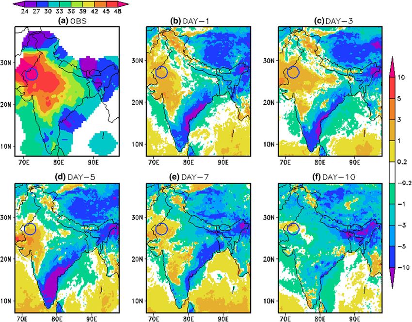
163       Page 2 of 11                                           J. Earth Syst. Sci. (2020)129:163

                                                            inherent model biases. We have chosen rainfall and
                                                            air temperature at 2 m for the purpose as they are
                                                            most important parameters aAecting society.
                                                            Among the meteorological variables, rainfall is
                                                            most difBcult to forecast and forecast of 2 m tem-
                                                            perature is aAected by complexity of lower
                                                            boundary conditions and topography, hence accu-
                                                            rate forecast of these variables from NWP models
                                                            require bias correction and post-processing proce-
                                                            dures (Fan and Dool 2011). To avoid model
                                                            inherent biases instead of absolute values, trends
                                                            relative to a threshold value from climatology is
                                                            used to investigate model’s predictability. Soil
                                                            moisture can aAect 2 m temperature and rainfall
                                                            through exchange of heat Cux between ground and
                                                            atmosphere. Surface temperature forecast are
                                                            strongly dependent on station elevations, geographic
                                                            locations and other meteorological conditions and
                                                            cold biases in 2 m temperature reported over moun-
                                                            tainous regions (Wyszogrodzki et al. 2013).

                                                            2. NWP model details

                                                            NGFS model of version 14.1.0 is used in this
                                                            study and re-forecasts are carried out at 00 UTC
                                                            daily. Model uses two-time level semi-implicit
                                                            semi-Lagrangian dynamics and a time step of
                                                            450 seconds is used in dynamics computations.
                                                            The semi-Lagrangian advection calculations and
                                                            physics are treated on a linear, reduced Gaussian
                                                            grid in the horizontal domain. Model uses
                                                            Gaussian grid of 3072 9 1536 grid points hori-
                                                            zontally and vertically 64 hybrid sigma pressure
                                                            levels and a time step of 225 seconds is used in
                                                            physics computations. Real-time global (RTG)
                                                            sea surface temperature (SST), daily sea ice
                                                            analysis and blended snow analysis is used for
                                                            lower boundary conditions over ocean. Moderate
                                                            resolution imaging spectro-radiometer (MODIS)
                                                            based land surface albedo scheme and interna-
                                                            tional geo-sphere biosphere programme (IGBP)
                                                            vegetation scheme is employed in the model.
                                                            Planetary boundary layer (PBL) scheme eddy-
                                                            diffusivity mass-Cux (EDMF) is used for strongly
                                                            unstable PBL, while GFS eddy-diffusivity coun-
                                                            ter-gradient parameterization is used for the
                                                            weakly unstable PBL. The land surface model
Figure 1. Mean absolute difference between forecast and     (LSM) Noah LSM has four soil layers (10, 30, 60,
observation in highest daily maximum 2 m surface tempera-   100 cm thick) and includes frozen soil physics,
ture (°C) for the years 1999–2018.                          new formulations for inBltration and runoA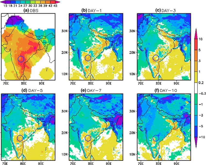
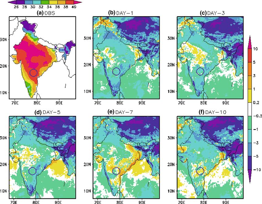
J. Earth Syst. Sci. (2020)129:163                                                                  Page 3 of 11 163

Figure 2. (a) Locations of stations where difference between forecast and observations are large, (b) mean difference between
forecast and observation (forecast–observation) (°C) before bias correction, and (c) mean difference between forecast and
observation (forecast–observation) (°C) after bias correction.

(giving more runoA for unsaturated soils), revised              3. Extreme temperature
physics of the snowpack and its inCuence on
surface heat Cux and albedo, tuning and addition                Prediction of extreme events gain more impor-
of canopy resistance parameters, spatially vary-                tance due to its impact on society and increase in
ing root depth, revised treatment of ground heat                frequency of occurrence of these events. Many
Cux and soil thermal conductivity, reformulation                recent studies suggested increase in occurrence of
for dependence of direct surface evaporation on                 heat wave events over land regions globally (Pai
Brst layer soil moisture and improved seasonality               et al. 2013; Rohini et al. 2016). In India also many
of green vegetation cover (GMTB 2018a). Mod-                    extreme heat events are reported in recent years.
iBed rapid radiative transfer model (RRTMG) is                  On May 19, 2016, in Phalodi, in northwest India,
used for parameterizing long wave and short                     maximum temperature recorded 51°C a new
wave radiation (GMTB 2018b). To mitigate the                    highest over India. In 2015 May, a severe heat
unresolved sub-grid cloud variability when deal-                wave event occurred in Andhra Pradesh and
ing multi-layered clouds, a Monte-Carlo inde-                   Telangana in southeast part of India. Although
pendent column approximation (McICA) method                     heat wave events are increasing over India, no
is used in the RRTMG radiation transfer com-                    positive trends are observed in occurrence of
putations. In addition to the major atmospheric                 highest maximum temperature of the year in most
absorbing gases of ozone, water vapour, and                     of India since the 1970s (Van Oldenborgh et al.
carbon dioxide, the algorithm also includes var-                2018). In India, heat wave events occur during the
ious minor absorbing species such as methane,                   period April to June. Different indices are used for
nitrous oxide, oxygen, and up to four types of                  identifying extreme temperature events (Casa-
halocarbons (CFCs). Scale and aerosol aware                     nueva et al. 2013). In the studies of extreme heat
deep and shallow convective parameterization is                 events, 90th percentile of daily maximum tem-
employed for representing convection (White                     perature is used as an index for identifying
et al. 2018).                                                   extreme events (Hamilton et al. 2012; Rohini
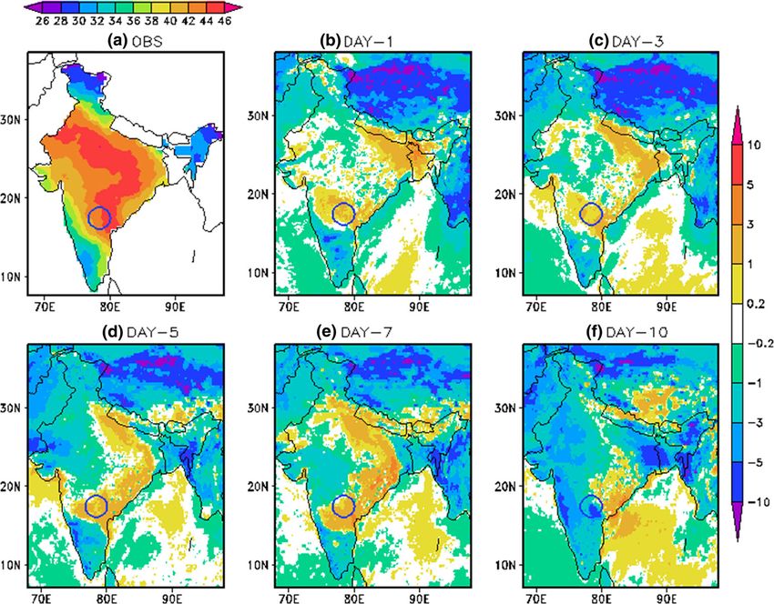
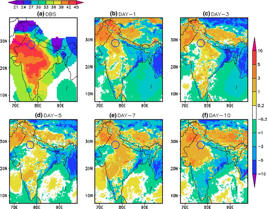
163      Page 4 of 11                                         J. Earth Syst. Sci. (2020)129:163

et al. 2016). Heat waves are considered as               used to compare the forecasts. Predictability of
anomalous episodes of extremely high tempera-            model in forecasting these events are assessed rel-
tures lasting for several days, incurring wide-          ative to a threshold value estimated using 20 yrs
spread devastating impacts. According to the             climatology prepared from re-forecasts. A thresh-
criteria speciBed by IMD, if climatological maxi-        old value of 90th percentile is used as a reference to
mum temperature is above 40°C, a departure of            identify extreme events and different threshold
5–6°C is considered as heat wave, while if clima-        values are computed for forecasts of different lead
tological maximum temperature is below 40°C, a           times. Cases with the temperature above threshold
departure of 4–5°C is considered as heat wave. In        are considered as unusually warm. The difference
inland stations, heat wave is declared if maximum        between model forecasts of different lead times
temperature is above 45°C, while in coastal sta-         with their respective threshold values is used for
tions if maximum temperature is above 40°C               identifying extreme events. A positive differ-
(Sandeep and Prasad 2018).                               ence between the forecast and threshold (Forecast–
   Heat wave episodes over Indian region usually         Threshold) indicates extremeness of an event in
occur in the months of May and June (Pai et al.          re-forecasts.
2013; Umakanth et al. 2019). In order to Bnd the            Figure 3 shows maximum temperature observa-
capability of re-forecasts in identifying extreme        tions and forecast differences relative to respective
temperature over different regions, daily maximum        threshold corresponds to 2016 May 19, the day on
surface air temperature data from IMD synoptic           which extreme temperature is reported in Phalodi
stations (Srivastava et al. 2009) is compared with       in Rajasthan in northwest India. The location of
model forecasts of lead times 24 hr, 72 hr and 120       interest is marked by blue circle. It can be seen
hr. At each station, highest temperature recorded        from different plots that maximum temperature
each day in the period 1999–2018 is identiBed for        above 90th percentile is predicted in all the fore-
the months of May and June and compared with             casts up to lead time of 10 days. On 2017 April
corresponding model forecasts. Figure 1 shows            20, heat wave conditions were reported in Delhi
mean difference between model and observations in        and adjacent places of Punjab and Haryana (Mo-
the forecasts of lead times day1, day3 and day5 for      hapatra et al. 2018). Figure 4 shows the similar
the month of May and June. It is found that in 17        plot of maximum temperature corresponds to April
stations difference between model and observation        20, 2017 and region of interest is denoted by blue
is large ([2 K) and their locations are given in map     circle. It can be seen that extreme temperature is
(Bgure 2a). Figure 2(b) shows mean difference            predicted in all the forecasts up to lead time of 10
between model and observations and their stan-           days. In 2015 April–June months, Andhra Pradesh
dard deviation at these stations is with large dif-      and Telangana experienced extreme heat condi-
ference. We attempted bias correction of maximum         tions. A severe heat wave reported in 2015 May 21
temperature at these stations to eliminate model         to June 4 in Andhra Pradesh and Telangana
biases. Bias correction is performed by taking           region. We investigated extremity of event in
monthly mean of differences between model and            model forecasts for May 23, 2015 and correspond-
observation of that particular station in respective     ing plot is shown in Bgure 5. It can be seen that
years. Figure 2(c) shows bias corrected mean dif-        model is able to predict extreme conditions up to
ference and standard deviation of maximum tem-           168 hr lead time. In 2015, April 15–May 30 heat
perature at these stations. These stations are either    wave event is reported in Hyderabad with mean
situated at higher altitudes or at coastal regions. In   temperature of 39.9° (NDMA guidelines 2016). We
orographic regions, capturing the spatial variation      investigated temperature over Hyderabad region
of near surface temperature represents a significant     during the period and plot for same for 23rd April
challenge to forecasting. Temperature varies with        2015 can be seen in Bgure 6. Although high tem-
height due to the background air mass lapse rate         perature remained in the region for several days, on
and, in addition, temperatures may be further            considering magnitude it does not qualify unusu-
depressed in valleys due to the formation of cold air    ally warm event based on our criteria. On 23rd
pools (Sheridan et al. 2010).                            April years 2001, 2009, 2008, 2016 and 2011 are
   In this section, some of the high temperature         warmer than 2015 in the region. In 2016 April,
events reported in India in recent years are inves-      extreme temperature is reported in many parts of
tigated. The daily gridded maximum temperature           Andhra Pradesh and Telangana and plot corre-
observation over Indian region provided by IMD is        sponds to April 23rd 2016 is shown in Bgure 7. In
J. Earth Syst. Sci. (2020)129:163                                                                      Page 5 of 11 163

Figure 3. 2016 May 19, maximum temperature (°C) observations and difference between forecast and threshold (forecast–
threshold) for the lead times day1, day3, day5, day7 and day10. The region Phalody, extreme temperature reported is marked in blue
circle.

Figure 4. 2017 April 20, maximum temperature (°C) observations and difference between forecast and threshold (forecast–
threshold) for the lead times day1, day3, day5, day7 and day10. The region Delhi and adjacent region, extreme temperature reported
is marked in blue circle.
163        Page 6 of 11                                               J. Earth Syst. Sci. (2020)129:163

Figure 5. 2015 May 23, maximum temperature (°C) observations and difference between forecast and threshold (forecast–
threshold) for the lead times day1, day3, day5, day7 and day10. Hyderabad and adjacent region, extreme temperature reported is
marked in blue circle.

Figure 6. 2015 April 23, maximum temperature (°C) observations and difference between forecast and threshold (forecast–
threshold) for the lead times day1, day3, day5, day7 and day10. Hyderabad and adjacent region, extreme temperature reported is
marked in blue circle.
J. Earth Syst. Sci. (2020)129:163 Page 7 of 11 163
Figure 7. 2016 April 23, maximum temperature (°C) observations and difference between forecast and threshold (forecast–
threshold) for the lead times day1, day3, day5, day7 and day10. Hyderabad and adjacent region, extreme temperature reported is
marked in blue circle.
Bgure 7, it can be seen that extreme event is be seen that extreme rainfall is predicted up to day3
predicted in re-forecasts up to lead time of day7. forecast. Similar plot for August 15 can be seen in
Bgure 9. The extremeness of rainfall event over the
4. Extreme rainfall region can be seen in all forecasts and pattern is
exactly matching up to day5 forecast. In August
Increasing trend in the frequency of occurrence 2019 also Kerala received heavy rainfall. Plots cor-
extreme rainfall events over the Indian region is respond to August 8th 2019 is shown in Bgure 10. It
reported by many researchers (Goswami et al. 2006; can be seen that extremeness of event is predicted in
Roxy et al. 2017). Due to large variability in rainfall all the forecasts. On 2013 June 17, Uttarakhand in
pattern, different thresholds are used at different north India received heavy rainfall and corre-
regions. In this study, one standard deviation above sponding plots are given in Bgure 11. Here
mean climatology is used as threshold for identifying extremeness of event is predicted in re-forecasts up
extreme rainfall and daily threshold value is com- to lead time of 3 days.
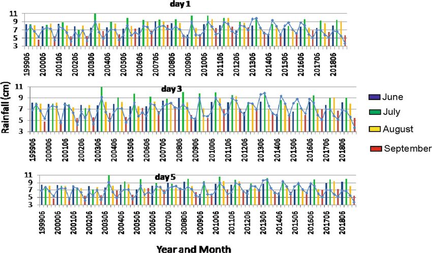
puted for different lead times using retrospective Monthly mean of rain fall observations and fore-
forecasts. Some extreme rainfall events reported in casts during the southwest monsoon period
recent past is investigated with same methodology June–September are compared to Bnd out model’s
adopted in case of temperature (forecast–threshold). ability to predict general pattern. Figure 12 shows
On 2018 August 2, spells of heavy rainfall occurred in monthly mean of observations (line plot) and fore-
Kerala in south India during August 15–17 and casts of different lead times for the period 1999–2018.
August 8–9. In this study, IMD NCMRWF (Mitra Main features of rainfall during this period like
et al. 2009) gridded rainfall data combining rain drought in 2002 July, drought in 2009 June, excess
gauge and satellite derived rainfall is used for com- rainfall in July 2003, excess rainfall in August 2011
paring forecasts. Figure 8 shows the rainfall obser- can be identiBed from the plots. Although there is no
vations and difference between forecasts of different exact match exists between magnitude of observa-
lead times with their respective threshold (fore- tion and forecasts, the trends can be identiBed.
cast–sthreshold) corresponds to August 9th. It can Figure 13 shows 20 yrs mean seasonal rainfall for the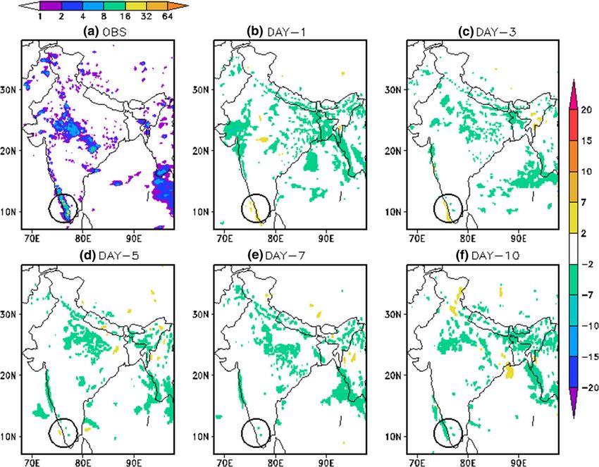
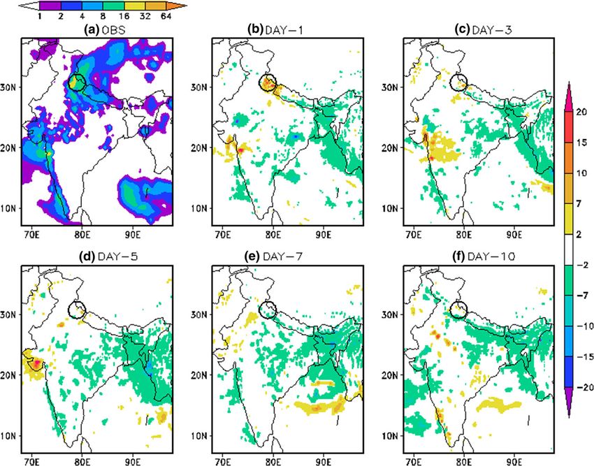
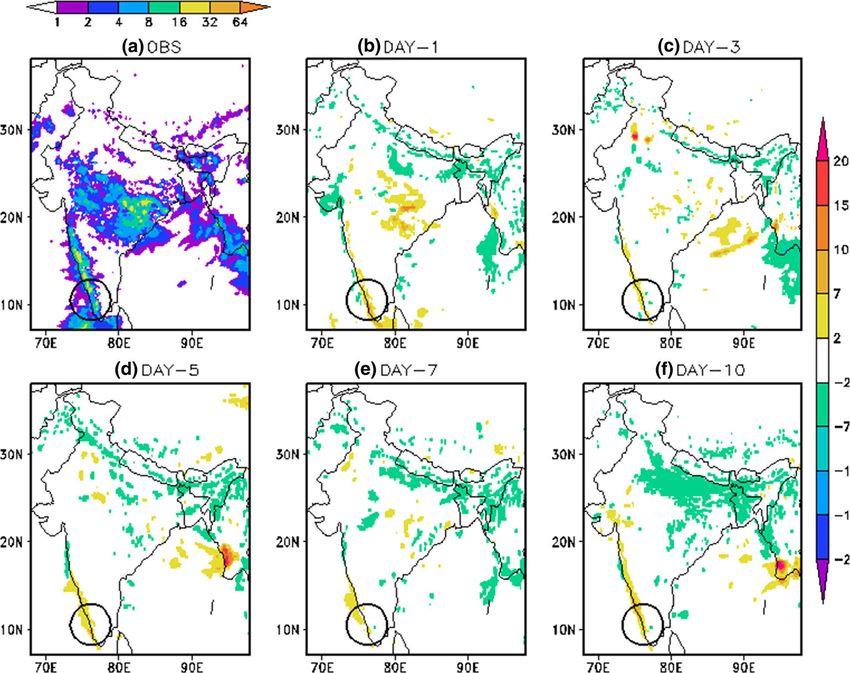
163        Page 8 of 11                                                 J. Earth Syst. Sci. (2020)129:163

Figure 8. 2018 August 9, 24 hr accumulated rainfall (cm) observations and difference between forecast and threshold
(forecast–threshold) for the lead times day1, day3, day5, day7 and day10. Kerala region, heavy rainfall experienced is marked in
black circle.

Figure 9. 2018 August 15, 24 hr accumulated rainfall (cm) observations and difference between forecast and threshold
(forecast–threshold) for the lead times day1, day3, day5, day7 and day10. Kerala region, heavy rainfall experienced is marked in
black circle.
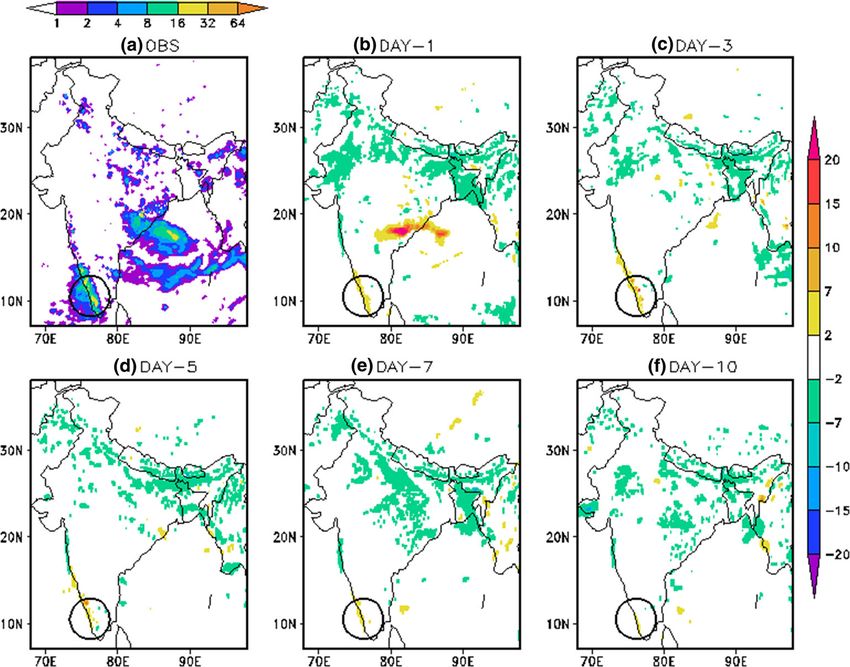
J. Earth Syst. Sci. (2020)129:163                                                                    Page 9 of 11 163

Figure 10. 2019 August 8, 24 hr accumulated rainfall (cm) observations and difference between forecast and threshold
(forecast–threshold) for the lead times day1, day3, day5, day7 and day10. Kerala region, heavy rainfall experienced is marked in
black circle.

Figure 11. 2013 June 17, 24 hr accumulated rainfall (cm) observations and difference between forecast and threshold
(forecast–threshold) for the lead times day1, day3, day5, day7 and day10. Uttarakhand region, heavy rainfall experienced is
marked in black circle.
163        Page 10 of 11                                               J. Earth Syst. Sci. (2020)129:163

Figure 12. Monthly mean of rainfall (cm) in observations (line plot) and forecasts (bar plot) of lead times day1, day3 and day5
during the months June–August from year 1999–2018.

Figure 13. Mean seasonal rainfall (cm) for JJAS period in forecasts (day1, day3, day5, day7, day9) and observed rainfall.

JJAS period in observations and forecasts of lead                events, and highest maximum temperature reported
times day1, day3, day5, day7 and day9. It is found               in different regions are used in investigating extreme
that there exists good match in mean rainfall                    temperature. In investigating extreme rain forecast,
between forecasts and observations, with a correla-              two rainfall events occurred in Kerala in 2018 and
tion value varying from 0.87 in day1 forecast to a               2019 August and extreme rainfall occurred in
correlation value of 0.82 in day9 forecasts.                     Uttarakhand in 2013 June is considered. Temporal
                                                                 pattern in monthly mean rainfall in months
5. Conclusions                                                   June–August during the period is investigated. It is
                                                                 found that re-forecast is able to predict the extreme
In this study, representation of some recent past                temperature events over the region with sufBcient
events of extreme temperature and rainfall in re-                lead time. In case of rain fall within shorter lead time
forecasts is investigated. Some of the heat wave                 (up to day3) model is able to forecast extreme events
J. Earth Syst. Sci. (2020)129:163 Page 11 of 11 163
accurately, but accuracy decreases as lead time improving heat wave warning over India; Report No: FDP/
increases. IdentiBed biases in prediction of highest HW/1/2017 National Weather Forecasting Centre, New
Delhi, IMD.
maximum temperature at some stations in hilly
Mukhopadhyay P, Prasad V S, Krishna R P, Deshpande M,
regions and some coastal stations. On implementing Ganai M, Tirkey S, Sarkar S, Goswami T, Johny C J, Roy
bias correction methods, forecasts are improved. K, Mahakur M, Durai V R and Rajeevan M 2019 Perfor-
General pattern of the rainfall over the region during mance of a very high-resolution global forecast system
the period is represented well in the re-forecasts. model (GFS T1534) at 12.5 km over the Indian region
during the 2016–2017 monsoon seasons; J. Earth Syst.
Sci. 128(155) 1–18, https://doi.org/10.1007/s12040-019-
1186-6.
Acknowledgement NDMA 2016 Guidelines for preparation of action plan –
Prevention and management of heat-wave; Government of
Authors are thankful to Head, NCMRWF for the India, https://ndma.gov.in/images/guidelines/guidelines-
support provided in executing this work. heat-wave.pdf.
Pai D S, Smitha A and Ramanathan A N 2013 Long term
climatology and trends of heat waves over India during the
recent 50 years (1961–2010); Mausam 64(4) 585–604.
References Prasad V S, Johny C J, Mali P, Sanjeev K S and Rajagopal E
N 2017 Retrospective analysis of NGFS for the years
Casanueva A, Herrera S, Fern andez J, Frıas M D and 2000–2011; Curr. Sci. 112(2) 370–377.
Guti errez J M 2013 Evaluation and projection of daily Rohini P, Rajeevan M and Srivastava A K 2016 On the
temperature percentiles from statistical and dynamical variability and increasing trends of heat waves over India;
downscaling methods; Nat. Hazards Earth Syst. Sci. 13 Sci. Rep. 6 26153, https://doi.org/10.1038/srep26153.
2089–2099. Roxy M K, Ghosh S and Pathak A et al. 2017 A three-fold rise
Fan Y and van den Dool H 2011 Bias correction and forecast in widespread extreme rain events over central India;
skill of NCEP GFS ensemble week-1 and week-2 precipita- Nat. Commun. 8 708, https://doi.org/10.1038/s41467-017-
tion, 2-m surface air temperature, and soil moisture 00744-9.
forecasts; Wea. Forecasting 26 355–370. Sandeep A and Prasad V S 2018 Intra-annual variability of
GMTB 2018a GFS Noah Land surface model; GMTB Com- heat wave episodes over the east coast of India; Int.
mon Community Physics Package (CCPP) ScientiBc Doc- J. Climatol. 38(1) 617–628, https://doi.org/10.1002/joc.
umentation Version 1.0 NCAR and NOAA/GSD, https:// 5395.
dtcenter.org/gmtb/users/ccpp/docs/sci˙doc/group˙noah˙ Sheridan P, Smith S, Brown A and Simon Vosper A S 2010
l˙s˙m.html. Simple height-based correction for temperature downscal-
GMTB 2018b GFS RRTMG shortwave/longwave radiation ing in complex terrain; Meteorol. Appl. 17 329–339.
scheme; GMTB Common Community Physics Package Srivastava A K, Rajeevan M and Kshirsagar S R 2009
(CCPP) ScientiBc Documentation Version 1.0 NCAR Development of a high resolution daily gridded temperature
and NOAA/GSD, https://dtcenter.org/gmtb/users/ccpp/ data set (1969–2005) for the Indian region; Atmos. Sci. Lett.
docs/sci˙doc/GFS˙RRTMG.html. 10 249–254, https://doi.org/10.1002/asl.232.
Goswami B N, Venugopal V, Sengupta D, Madhusoodanan M Umakanth N, Satyanarayana G C, Lakshmi H, Shweta C and
S and Xavier P 2006 Increasing trend of extreme rain events Akhil C 2019 Satellite and AWS based scrutiny of heat
over India in a warming environment; Science 314 wave over AP; Int. J. Recent Technol. Eng. (IJRTE) 8(4)
1442–1445, https://doi.org/10.1126/science.113202. 4719–4722.
Hamill T M, Whitaker J S and Mullen S L 2006 Reforecasts: Van Oldenborgh G J, Philip S, Kew S, Van Weele M, Uhe P,
An important new data set for improving weather predic- Otto F, Singh R, Pai I, Cullen H and Achutarao K 2018
tions; Bull. Am. Meteor. Soc. 87 33–46. Extreme heat in India and anthropogenic climate change;
Hamilton E R, Eade R J, Graham A A, Scaife D M, Smith A M Nat. Hazards Earth Syst. Sci. 18 365–381, https://doi.org/
and MacLachlan C 2012 Forecasting the number of extreme 10.5194/nhess-18-365-2018.
daily events on seasonal timescales; J. Geophys. Res. 117 White G, Yang F and Tallapragada V 2018 The Development
D03114, https://doi.org/10.1029/2011JD016541. and Success of NCEP’s Global Forecast System; National
Mitra A K, Bohra A K, Rajeevan M and Krishnamurti T N Centers for Environmental Prediction: National Oceanic
2009 Daily Indian precipitation analyses formed from a and Atmospheric Administration, USA.
merge of rain-guage with TRMM TMPA satellite derived Wyszogrodzki A A, Liu Y, Jacobs N, Childs P, Zhang Y, Roux
rainfall estimates; J. Meteorol. Soc. Japan 87A 265–279. G and Warner T T 2013 Analysis of the surface temper-
Mohapatra M, Sushma N, Naresh K, Charan S, Sathidevi, ature and wind forecast errors of the NCAR-AirDat
Bhan S C, Durai V R and Joardar D 2018 Implementation operational CONUS 4-km WRF forecasting system; Mete-
report 2017: Forecast demonstration project (FDP) for orol. Atmos. Phys. 22 125–143.
Corresponding editor: A K SAHAIYou can also read