Use of CALIPSO lidar observations to evaluate the cloudiness simulated by a climate model

Use of CALIPSO lidar observations to evaluate the cloudiness simulated by a climate model

H. Chepfer(1), S. Bony(1), D. Winker(3), M. Chiriaco(2), J­L. Dufresne(1),, G. Sèze(1)

       (1)
          LMD/IPSL, CNRS and Université Pierre et Marie Curie, Paris, France
       (2)
          NASA/LaRC, Hampton, Virginia, USA.
       (3)
          SA/IPSL, CNRS and Université Versailles­Saint Quentin, France

Abstract:

New space­borne active sensors make it possible to observe the three­dimensional structure of clouds. Here we
use CALIPSO lidar observations together with a lidar simulator to evaluate the cloudiness simulated by a climate
model: modeled atmospheric profiles are converted to an ensemble of subgrid­scale attenuated backscatter lidar
signals from which a cloud fraction is derived. Except in regions of persistent thick upper­level clouds, the cloud
fraction diagnosed through this procedure is close to that actually predicted by the model. A fractional cloudiness
is diagnosed consistently from CALIPSO data at a spatio­temporal resolution comparable to that of the model.
The comparison of the model’s cloudiness with CALIPSO data reveals discrepancies more pronounced than in
previous model evaluations based on passive observations. This suggests that space­borne lidar observations
constitute a powerful tool for the evaluation of clouds in large­scale models, including marine boundary­layer
clouds.

1. Introduction
Clouds are the primary modulators of the Earth's radiation budget and still constitute the main source of
uncertainty in model estimates of climate sensitivity [Randall et al. 2007]. Clouds simulated by climate models
have long been evaluated using passive remote­sensing [e.g. Zhang et al. 2005], making the vertical structure of
clouds difficult to assess. With the new generation of satellites carrying cloud profiling radar and lidar
instruments such as CloudSat [Stephens et al. 2002], ICESat/GLAS [Spinhirne et al. 2005] and
CALIOP/CALIPSO [Winker et al. 2007] a near­global view of the three­dimensional distribution of clouds
becomes possible. However, to make the comparison between modeled clouds and these observations
meaningful, it is necessary to take into account the effects of cloud overlap, spatial resolution, and active signal
attenuation.
For this purpose, we propose a methodology of comparison of CALIOP/CALIPSO lidar data with modeled
clouds that is intermediate between “model­to­satellite” [Morcrette 1991, Doutriaux­Boucher et al. 1998,
Chiriaco et al. 2005, Chepfer et al. 2007] and “satellite­to­model” approaches: grid­scale model outputs are
converted to an ensemble of subgrid­scale lidar signals while high­resolution CALIPSO lidar signals are
averaged to the model vertical resolution , and then a cloud fraction is diagnosed from these signals similarly for
model and for observations.
The lidar simulator is described in Section 2, the processing of CALIPSO data is presented in Section 3 and the
cloud detection method in Section 4. The methodology of model­data comparison is then applied to the general
circulation model (GCM) LMDZ4 [Hourdin et al. 2006], and the results are presented in Section 5.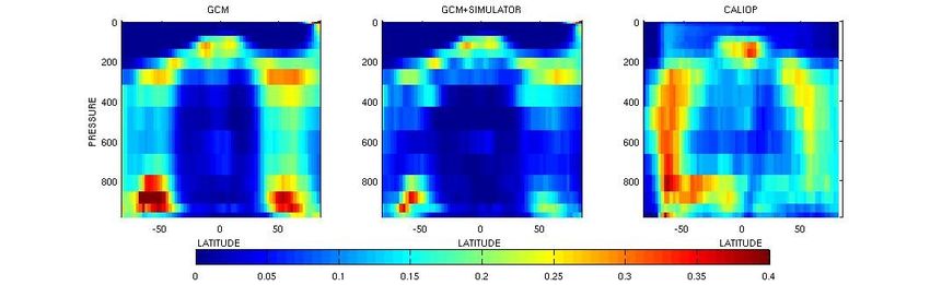

2. Simulation of lidar profiles from climate model outputs

2.1. Lidar equation
Our aim is to diagnose from climate model outputs the lidar profiles that would be observed by CALIPSO if the
satellite was flying above an atmosphere similar to that predicted by the model. At the wavelength of the
CALIOP/CALIPSO lidar (λ = 532 nm), atmospheric cloud particles and gas molecules contribute to scattering
but not to absorption. In these conditions, the lidar ATtenuated Backscattered (ATB) signal corrected of
geometrical effects and normalized to the molecular signal is given by :
                                                              z
                                                     − 2η    ∫ ( α sca, part (z)+   sca,mol   (z)).dz
                                                                                                        (1)
ATB(z) = (        sca, part (z) +   sca,mol (z)).e
                                                            z TOA

where βsca,part , βsca,mol are lidar backscatter coefficients [m­1sr­1] and αsca,part , αsca,mol attenuation coefficients [m­1] for
particles and molecules, and η is a multiple scattering coefficient [Chiriaco et al. 2005].
The molecular properties (βsca,mol and αsca,mol) are computed from Collis and Russel [1976] as a function of
temperature and pressure. The particle backscattered coefficient βsca,part is linked to the attenuation coefficient α
sca,part and the backscatter­to­extinction ratio kpart [sr ] through :
                                                          ­1

   sca, part (z) = k part (z). sca, part (z)                                                     (2)
 sca, part   (z) = ∫ πr2Q(r)n(r, z)dr                                                                         (3)
and kpart = P(π)/4π, where r is the particle radius, n(r,z) the particle size distribution, P(π) the backscattering phase
function and Q(r) the scattering efficiency. To be consistent with the GCM, we assume that the cloud particles
are spherical. Therefore, P(π) is parameterized as a function of the effective radius using Mie theory and, as most
of the cloud particles are larger than λ = 532nm, Q(r) is set to 2.
The multiple scattering coefficient (η) is variable in space and time as a function of the lidar footprint diameter,
and the size, shape and density of the particles in the atmosphere. Theoretically it ranges between 0 and 1, but for
CALIOP it is about 0.7 in ice clouds and less in water clouds [Winker et al. 2003]. Here we use η=0.7 and check
the sensitivity of the results to this value in section 5.
To highlight the contribution of particles to the lidar signal, it is common to consider the scattering ratio SR(z),
defined as the ratio of the total ATB signal (Equation 1) over the molecular ATB signal (which is the ATB signal
in the absence of particules, i.e. when αsca,part(z)=0). SR(z) is equal to 1 in the absence of particles (gas molecules
only) and, when the lidar signal is not attenuated, is greater than unity in the presence of particles.

2.2. Application to GCM outputs
The LMDZ4 GCM has an horizontal resolution of 2.5° in latitude, 3.75° in longitude, and is discretized into 19
vertical levels [Hourdin et al. 2006]. In each gridbox, the model calculates the vertical profiles of temperature,
pressure, cloud fraction (assuming a maximum­random overlap), cloud condensate and effective radius of cloud
droplets and ice crystals. These profiles are converted to an ensemble of subgrid­scale profiles by dividing each
gridbox into 50 subcolumns generated stochastically using the Subgrid Cloud Overlap Profile Sampler [Klein
and Jakob 1999; Webb et al. 2001] : in each subcolumn, the cloud fraction is assigned to be 0 or 1 at every model
level, with the constraint that the cloud condensate and cloud fraction averaged over all subcolumns is consistent
with the grid­averaged model diagnostics and the cloud overlap model assumption.
In each subcolumn, the particle backscatter coefficient βsca,part and the attenuation coefficient αsca,part are the sums
of liquid and ice cloud particles coefficients (aerosols are not considered in this study). They are computed from
equations (2) and (3) after the model mixing ratios of in­cloud liquid and ice water content have been converted

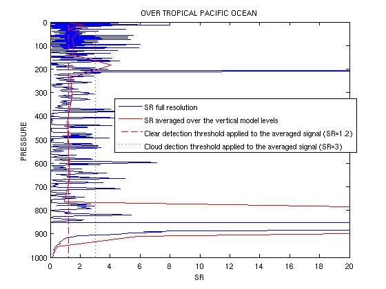
to particle concentrations. This is done by assuming that the cloud particles are spherical with a radius equal to
the effective radius predicted by the model. Finally, equation (1) is used to compute in each subcolumn of each
gridbox the molecular and total ATB lidar profiles, and hence the SR profile.

3. CALIPSO observations
The CALIOP lidar, that operates at 532 and 1064 nm, was launched in April 2006 on­board the helio­synchro­
neous CALIPSO platform [Winker et al. 2007]. This study uses the total ATB measurements derived from the
Version 1.10 Level 1 CALIOP dataset collected at 532 nm during night time from January to March 2007. The
horizontal and vertical resolutions of these measurements are 333 m (333 m along track and 75 m cross track)
and 30 m (respectively) below 8 km, and 1 km and 60 m at higher altitudes.
At each time and location, a molecular ATB profile is computed by using GMAO (Global Modeling and Assimil­
ation Office) temperature and pressure profiles [Bey et al. 2001]. This profile is normalized (scaled) so as to
match the Level 1 ATB profile measured between 27 and 29 km, where the atmosphere is free of particles, and
then the scattering ratio (SR) is inferred by dividing the measured ATB profile by this molecular profile.
Then, we reduce the vertical resolution of the CALIOP ATB profiles to that of the GCM (19 pressure levels) by
vertical averaging. This makes the vertical resolution of CALIPSO profiles consistent with that of model compu­
tations and strongly increases the signal­to­noise ratio of the lidar signals (section 4 and supplementary material).

4. Cloud diagnostics
The presence of cloud layers is then diagnosed consistently for the model and for observations from the vertical
profile of lidar SR. For each CALIOP/CALIPSO profile or model subcolumn, we use different SR thresholds to
label each atmospheric layer as “clear” (if 0.01 < SR ≤ 1.2), “cloudy” (if SR ≥ 3 of if the layer is the first fully
attenuated layer encountered from top), “unclassified” (if 1.2 < SR < 3) or “fully attenuated” (if SR ≤ 0.01). The
latest flag is set when optically thick clouds occurring in upper layers obscure the layers below and fully
attenuate the laser beam. The conversion of SR in terms of optical depth depends on many factors. As an
informal guesstimate, an SR value around 3 may be obtained with a liquid water cloud of 250­500m depth,
having a cloud optical depth of 0.015 ­0.03 and a liquid water path of 0.1­0.2 g/m2.
The main cloud layers (which are associated with the largest SR values in the full resolution CALIOP profile) are
detected by applying these thresholds to the vertically averaged CALIOP profile, but the optically thin cloud
layers such as subvisible cirrus clouds and potentially some semi­transparent clouds can be labelled as
“unclassified” (Supplementary Material). This illustrates that the detection of a cloud layer obviously depends on
the criteria used for this detection. Advanced algorithms of cloud fraction retrieval such as those used for level 2
CALIOP products would provide a better detection of the different cloud layers (especially of the optically
thinnest and subvisible ones) and thus would likely report larger cloud fractions than our simple detection
method. Although this is not critical for this model­data comparison study because the cloud layers are diagnosed
similarly in the model and in observations, this implies that our study ignores the optically thinnest cloud layers
which may not be detected (in simulations like in observations) by our simple cloud detection criteria. Then, a
“lidar­derived cloud fraction” is computed for each vertical level at the resolution of the model grid­box as the
ratio of the number of “cloudy” layers (or profiles) encountered within this grid­box over the total number of
layers that are not “fully attenuated”. Layered cloud fractions are also computed for three atmospheric layers :
upper levels (between the 50 and 440 hPa pressure levels), middle levels (between 440 and 680 hPa) and low
levels (altitudes below the 680 hPa level).

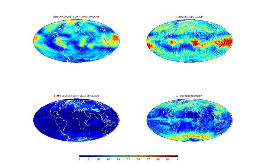
5. Results

5.1. Model cloud fractions diagnosed from the lidar simulator.
The lidar simulator described in section 2 is applied to daily atmospheric profiles derived from a LMDZ4
simulation forced by observed sea surface temperatures. The daily cloud fractions diagnosed from the simulator
are then averaged in time to produce a monthly­mean CALIPSO­like cloud fraction.
Sensitivity calculations indicate that the frequency of the model inputs and simulator calculations (once a day,
every 3 hour, 1.5 hour or 30 min), as well as the value of the multiple scattering coefficient assumed in the
simulator (e.g. using η = 0.3 instead of η = 0.7) have negligible impacts (less than 1 %) on the monthly mean
CALIPSO­like cloud fraction (not shown). Using a different threshold (e.g. SR≥ 5 instead of SR≥ 3) does not
change drastically the results neither, which suggests that the model does not simulate many optically thin clouds.
The layered cloud fractions derived from the lidar simulator and the simple cloud detection method are first
compared to the cloud fractions originally predicted by the GCM. The CALIPSO­like cloud fractions (Figures
1b) are generally close to their original counterpart (Figures 1a),. Since the attenuation of the backscattered lidar
signal at a given height depends on the presence of overlapping clouds at higher altitudes, such a result is
expected at upper levels but not necessarily at lower levels. As shown by zonal means (Figures 2 a­b), the
original and CALIPSO­like cloud fractions at low and middle­levels differ mainly in regions of persistent
convective activity (such as in the inter­tropical and southern­pacific convergence zones and over the warm pool)
and in extratropical regions associated with frontal cloudiness. However, over a large fraction of the Earth, the
simulated upper­level clouds are either not optically thick enough (the laser is typically attenuated when the
optical depth is larger than 3) or not frequent or not persistent enough to obscure the view of low atmospheric
layers from above. Despite the lidar attenuation effects, the CALIPSO simulator thus constitutes a powerful tool
to diagnose and then to evaluate the different cloud types predicted by the GCM, including marine boundary
layer clouds.
Before the era of space­borne active remote sensing, GCM clouds were evaluated mostly against passive
observations using the International Cloud Climatology Project (ISCCP) simulator [Klein and Jakob 1999, Webb
et al. 2001. Zhang et al. 2005]. When applied to our GCM, the ISCCP and CALIPSO simulators both diagnose
an upper­level cloud fraction that resembles that originally predicted by the GCM (not shown). However, the
low­level cloud fraction diagnosed from the CALIPSO simulator (Figure 1b) is much closer to that predicted by
the GCM (Figure 1a) than that derived from the ISCCP simulator (Figures 1c).

5.2. Cloud fractions derived from CALIPSO observations.
The layered and zonal mean vertical distributions of the cloud cover diagnosed from CALIPSO data using the
methodology discussed in sections 3 and 4 are shown in Figures 3c­d, 1d, and 2c respectively. As expected for
the January­February­March season, the upper level cloud fraction exhibits maxima in deep convective regions
located over tropical land areas, over the maritime continent and the pacific warm pool and over the southern­
pacific convergence zone. Secondary maxima occur at extra­tropical latitudes. Middle­level clouds occur in
middle­latitudes and in regions of deep convection. CALIPSO data suggest that low­level clouds occur nearly
everywhere over ocean. Maximum low­level cloud fractions are found at subtropical latitudes, at the eastern side
of the ocean basins which are known to be covered by stratus and stratocumulus clouds, but cloud fractions of 40
to 60 % are also reported over the tropical trade winds and at middle latitudes. Note that owing to the pronounced
diurnal cycle of oceanic tropical low clouds [Rozendaal et al. 1995], these nightime values might be higher than
daytime or diurnally averaged values.

Sensitivity tests using the CALIPSO lidar color ratio to detect the presence of aerosols (defined as cases where
the ratio between the ATB measured at 1064 and 532 nm exceeds 0.6, [Liu et al. 2005]) show that the cloud
detection criteria defined in section 4 do not misinterpret the presence of aerosols as low­level clouds :
atmospheric layers with large aerosol burden, such as over Africa or over ocean regions west of the Sahara, are
labelled as “unclassified”. On the other hand, other tests show that the cloud fraction reported in the trades
critically depends on the SR threshold used for cloud detection (e.g. it is substantially reduced when the threshold
is changed from 3 to 5), while it is not the case at the eastern side of the ocean basins or in the extratropics. This
suggests that the large cloud fractions reported in the trades are related to the ability of lidar measurements to
detect optically thin or small broken clouds owing both to their high horizontal resolution and to their high
sensitivity to the presence of cloud particles., This is corroborated by the cloud fractions derived from
ICESat/GLAS lidar measurements (level 2 dataset, GLA09, release 26, Palm et al. 2002) on October and
November 2003 which are of same order of magnitude as those derived from CALIPSO at the same season (not
shown). The difficulty of detecting thin or/and broken low­level clouds with passive remote sensing [Turner et
al. 2007] presumably explains why data from the International Cloud Climatology Project [ISCCP, Rossow and
Schiffer 1999] report substantially smaller low­level cloud fractions (Figure 1e).

5.3. Evaluation of the GCM cloudiness against CALIPSO observations.
The comparison of the cloud fraction derived from the lidar simulator with that derived from CALIPSO
observations reveals large biases in the cloudiness simulated by the GCM (Figures 1, 2 and 3). The upper­level
cloud fraction is underestimated by several tens of % in the tropical deep convective regions and the middle­level
cloudiness is systematically underestimated, especially in the inter­tropical convergence zone (ITCZ) and in
middle­latitude regions associated with frontal clouds. But the largest biases appear for the low­level cloud
fraction, which is strongly overestimated (by about 25 %) over mid­latitude oceans and is strongly
underestimated (by up to a factor of 4) in the subtropics, both over the cold waters at the eastern side of the
Pacific, Atlantic and Indian oceans, and offshore over the subtropical oceans. Except in mid­latitudes and in the
ITCZ, these biases are unlikely to result from the attenuation of the lidar signal by overlapping optically thick
clouds (section 5.1).
Both in the tropics and in middle latitudes, the model­data discrepancies revealed by this comparison are more
pronounced than in previous comparisons using ISCCP observations and the ISCCP simulator (Figure 1) This
suggests that using space­borne lidar observations to evaluate large­scale models will help to point out systematic
biases in the cloudiness predicted by the models, especially in the simulation of marine boundary­layer clouds.

6. Conclusion
This paper proposes a methodology to evaluate the cloud fraction simulated by a GCM using space borne lidar
observations : on the one hand, the atmospheric profiles predicted by the GCM are converted (through a lidar
simulator) to an ensemble of subgrid­scale lidar signals similar to those observed from space; on the other hand,
the high vertical resolution of the lidar profiles measured by CALIOP/CALIPSO is degraded down to the vertical
resolution of the GCM; then, a fractional cloudiness is diagnosed from the simulated or observed profiles of lidar
scattering ratio using simple and consistent criteria.
When applied to the LMDZ4 GCM, the CALIPSO­like cloud fraction derived from this methodology reproduces
well the cloudiness originally predicted by the model, and this despite the attenuation effect of the lidar signal
and whatever the assumed value of the multiple scattering coefficient. When applied to CALIPSO data, this
simple methodology efficiently detects the main cloud layers, does not misinterpret them with the presence of

aerosols, and provides cloud fraction estimates that are of same order of magnitude than those derived from the
IceSAT/GLAS level 2 dataset.
The comparison of the cloud fraction derived from the lidar simulator with that derived from CALIPSO data
reveals large biases in the GCM cloudiness, which are more dramatic than those pointed out previously using
passive observations. In particular, striking differences between GCM and CALIPSO observations (found for all
seasons, not shown) occur for the marine boundary­layer clouds observed over most of the subtropical oceans.
As the response of these clouds to climate change constitutes a key uncertainty for GCM estimates of climate
sensitivity [Bony and Dufresne 2005], it is of great importance to improve their representation in climate models.
Efforts to improve the parameterization of shallow clouds in LMDZ4 are under way [Rio and Hourdin 2008],
and the methodology presented in this paper will allow us to quantify the extent to which the simulated cloud
fraction is improved at the large scale.
This study thus shows the large potential of CALIPSO observations and of the lidar simulator for the evaluation
of clouds simulated by climate models. Within the framework of the Cloud Feedback Model Intercomparison
Project (CFMIP, http://www.cfmip.net), the lidar simulator will be applied to several other climate models to
examine inter­model differences and systematic biases in the simulation of clouds by GCMs. For this purpose,
the GCM oriented CALIOP dataset processed and used in this study will be made available to the modelling
community. A comparison between this dataset and the CALIOP Level 2 product is underway (both for nightime
and daytime data) and will be reported in a future paper.

Acknowledgments.
The authors thank Vincent Noel for fruitful discussions and for his help in the processing of CALIOP level 1
data, and to Ionela Musat for her help in GCM data processing. NASA, CNES, ICARE and Climserv are
acknowledged for giving access to the CALIOP/CALIPSO data. Constructive comments from two anonymous
reviewers greatly helped to improve the manuscript.

2. References
Bey, I., D. , at al., Global modeling of tropospheric chemistry with assimilated meteorology: Model description
     and evaluation, J. Geophys. Res., 106(D19), 23073­23096, 10.1029/2001JD000807, 2001.
Bony S and J­L Dufresne, 2005; Marine boundary layer clouds at the heart of tropical cloud feedback
     uncertainties in climate models, Geophys. Res. Lett., 32, No. 20, L20806, doi:10.1029/2005GL023851.
Collis R. T. and P. B. Russel, 1976: Laser Monitoring of the Atmosphere. Springer­Verlag, New York.
Chepfer H., M. Chiriaco, R. Vautard, J. Spinhirne : Evaluation of the ability of MM5 meso­scale model to
     reproduce optically thin clouds over Europe in fall using ICE/SAT lidar space­born observations, Month.
     Weath. Rev., 135, 2737–2753.
Chiriaco M., R. Vautard, H. Chepfer, M. Haeffelin, Y. Wanherdrick, Y. Morille, A. Protat, J. Dudhia, C. F. Mass,
     2006 : ‘ The ability of MM5 to simulate thin ice clouds : Systematic comparisons with lidar/radar and fluxes
     measurements’, Month. Weath. Rev., 134, 897­918.
Doutriaux­Boucher M., J. Pelon, V. Trouillet, G. Sèze, H. Le Treut, P. Flamant, and M.Desbois, 1998: Simulation
     of Satellite Lidar and Radiometer Retrievals of a GCM Three­Dimensional Cloud Dataset. J. Geophys. Res.,
     Vol. 103, N0.D20, pp 26,025­26,039.
Hourdin, F., et al., 2006: The LMDZ general circulation model: climate performance and sensitivity to
     parameterized physics with emphasis on tropical convection. Climate Dynamics, 19 (15), 3445­3482, DOI:
     10.1007/s00382­006­0158­0.
Klein S. A. and C. Jakob, 1999: Validation and sensitivities of frontal clouds simulated by the ECMWF model.
     Mon. Wea. Rev., 127, 2514­2531.
Liu, Z., A. H. Omar, Y. Hu, M. A. Vaughan and D. M. Winker, 2005: CALIOP Algorithm Theoretical Basis
     Document, Part 3: Scene Classification Algorithms, PC­SCI­202.
Palm S., W. Hart, and D. Hlavka, 2002: GLAS atmospheric data products. GLAS algorithms theoretical basis
     document. Version 4.2. Lanham, MD: Science Systems and Applications, Inc.
Platt C. M. R. 1973: Lidar and Radiometric Observations of Cirrus clouds. J. of Atmos. Sci., 30, 1191­1204.
Randall, D. A., K. M. Xu, R. J. C. Somerville, and S. Iacobellis, 1996 : Single column models and cloud
     ensemble models as links between observations and climate models, J. Clim., 9, 1683­1697.
Randall, D. A., et al., 2007 : Climate Models and Their Evaluation. In: Climate Change 2007: The Physical
     Science Basis. Contribution of Working Group I to the Fourth Assessment Report of the Intergovernmental
     Panel of Climate Change [Solomon et al. (eds.)]. Cambridge University Press. Cambridge.
Rio, C., and F. Hourdin, 2008: A Thermal Plume Model for the Convective Boundary Layer: Representation of
     Cumulus Clouds. J. Atmos. Sci., 65, 407–425.
Rossow, W. B., and R. A. Schiffer, 1999: Advances in understanding clouds from the ISCCP, Bull. Amer.
     Meteor. Soc., 80, 2261­2287.
Rozendaal, M., C. Leovy, and S. Klein, 1995: An observational study of diurnal variations of marine stratiform
     cloud. J. Clim., 8, 1795­1809.
Spinhirne, J. D., S. P. Palm, W. Hartd, D. Hlavka, and E. J. Welton, 2005: Cloud and aerosol measurements from
     the GLAS: Overview and initial results, Geophys. Res. Let., 32, L22S03, doi:10.1029/2005GL023507.
Stephens G. L., et al., 2002: The CloudSat mission and the A­train, Bull. Am. Meteo. Soc., 1771­1790.
Turner, D. D., et al., 2007: Thin liquid water clouds: their importance and our challenge, Bull. Amer. Meteor.
     Soc., 88, 177­190.
Webb M, C Senior, S Bony and J­J Morcrette, 2001: Combining ERBE and ISCCP data to assess clouds in three
     climate models, Climate Dynamics, 17, 905­922.

Winker, D. 2003: Accounting for Multiple Scattering in Retrievals from Space Lidar. in Lidar Multiple Scatter­
   ing Experiments, Proc. SPIE, vol. 5059, edited by C. Werner, U. Oppel, and T. Rother, pp. 128­139, SPIE,
   Bellingham, WA.
Winker D., W. Hunt, and M. McGill, 2007: Initial Performance Assessment of CALIOP, Geophys. Res. Lett., 34,
   L19803, doi:10.1029/2007GL030135.
Zhang M H, et al., 2005: Comparing Clouds And Their Seasonal Variations in 10 Atmospheric General
   Circulation Models With Satellite Measurements. J. Geophys. Res., 110, D15S02,
   doi:10.1029/2004JD005021.

Figure 1: Low­level cloud fractions averaged for the January­February­March season. (a) The cloud fractions
actually predicted by the GCM, (b) the cloud fractions derived from the lidar simulator and (d) from
CALIOP/CALIPSO observations using similar consistent criteria. Also reported at the bottom is (c) the low­level
cloud fraction derived from ISCCP­D2 data and (e) that diagnosed from the ISCCP simulator.

Figure 2: Vertical distribution of the zonally averaged cloud fraction for January­February­March:
a) Original cloud fraction predicted by the GCM; b) GCM cloud fraction diagnosed from the lidar simulator; c)
Cloud Fraction derived from CALIOP/CALIPSO data.

Figure 3: (Top) Upper­level and (bottom) middle­level layered cloud fractions averaged for the January­
February­March season. The cloud fractions derived from the lidar simulator (left panels) and from
CALIOP/CALIPSO observations (right panels) are diagnosed consistently by using similar criteria.

Supplementary Material

Figure 1: Example of 330m­horizontal Lidar Scattering Ratio (SR) profile observed by CALIOP/CALIPSO
during night time over Pacific ocean.