A calibration procedure which accounts for non-linearity in single-monochromator Brewer ozone spectrophotometer measurements
←
→
Page content transcription
If your browser does not render page correctly, please read the page content below
Atmos. Meas. Tech., 12, 271–279, 2019
https://doi.org/10.5194/amt-12-271-2019
© Author(s) 2019. This work is distributed under
the Creative Commons Attribution 4.0 License.

A calibration procedure which accounts for non-linearity
in single-monochromator Brewer ozone
spectrophotometer measurements
Zahra Vaziri Zanjani1 , Omid Moeini1 , Tom McElroy1 , David Barton1 , and Vladimir Savastiouk2
1 York    University, 4700 Keele Street, Toronto, Ontario, M3J 1P3, Canada
2 Full   Spectrum Science Inc., 112 Tiago Avenue, Toronto, Ontario, Canada

Correspondence: Zahra Vaziri Zanjani (zahra_vaziri@yahoo.com)

Received: 21 May 2018 – Discussion started: 21 May 2018
Revised: 13 November 2018 – Accepted: 20 November 2018 – Published: 15 January 2019

Abstract. It is now known that single-monochromator                   In a study done by Karppinen et al. (2015), a method for
Brewer spectrophotometer ozone and sulfur dioxide mea-             correcting stray light has been presented that uses an additive
surements suffer from non-linearity at large ozone slant col-      correction, which is determined via instrument slit character-
umn amounts due to the presence of instrumental stray light        ization and a radiative transfer model simulation and is then
caused by scattering within the optics of the instrument. Be-      applied to the single Brewer data (Karppinen et al., 2015).
cause of the large gradient in the ozone absorption spectrum       The European Brewer Network is also applying stray-light
in the near-ultraviolet, the atmospheric spectra measured by       corrections, which includes an iterative process that results
the instrument possess a very large gradient in intensity in       in correcting the single Brewer data to agree with double
the 300 to 325 nm wavelength region. This results in a signif-     Brewer data (Rimmer et al., 2018; Redondas et al., 2018).
icant sensitivity to stray light when there is more than 1000      The first model requires measurements of the slit function
Dobson units (DU) of ozone in the light path. As the light         and the latter method relies on a calibrated instrument, such
path (air mass) through ozone increases, the stray-light effect    as a double Brewer, to characterize the instrument and to de-
on the measurements also increases. The measurements can           termine a correction for stray light.
be of the order of 10 %, low for an ozone column of 600 DU            This paper presents a simple and practical method to cor-
and an air mass factor of 3 (1800 DU slant column amount),         rect for the effects of stray light, which includes a mathemat-
which is an example of conditions that produce large slant         ical model of the instrument response and a non-linear re-
column amounts.                                                    trieval approach that calculates the best values for the model
   Primary calibrations for the Brewer instrument are carried      parameters. The model can then be used in reverse to provide
out at Mauna Loa Observatory in Hawaii and Izana Obser-            more accurate ozone values up to a defined maximum ozone
vatory in Tenerife. They are done using the Langley plot           slant path. The parameterization used was validated using an
method to extrapolate a set of measurements made under a           instrument physical model simulation. This model can be ap-
constant ozone vertical column to an extraterrestrial calibra-     plied independently to any Brewer instrument and correct for
tion constant. Since the effects of a small non-linearity at       the effects of stray light.
moderate ozone paths may still be important, a better cal-
ibration procedure should account for the non-linearity of
the instrument response. Studies involving the scanning of a
laser source have been used to characterize the stray-light re-
sponse of the Brewer (Fioletov et al., 2000), but until recently
these data have not been used to elucidate the relationship
between the stray-light response and the ozone measurement
non-linearity.

Published by Copernicus Publications on behalf of the European Geosciences Union.
272                                                            Z. Vaziri Zanjani et al.: A non-linearity calibration for Brewer

1   Introduction                                                    placed by double Brewers, and therefore, new measurements
                                                                    may show a false increase in ozone column amounts due to
The Brewer spectrophotometer instrument is a diffraction-           the effect of lower stray light in the DBr, particularly for mea-
grating polychromatic spectrophotometer which produces              surements made at large solar zenith angles. In this paper a
monochromatic light at a set of six exit slits. It measures total   method is described that accounts for the effect of stray light
column amounts of ozone, sulfur dioxide and aerosol optical         in the data from the SBr to provide more accurate, repro-
thickness (Silva and Kirchhoff, 2004) by direct sun measure-        cessed SBr data.
ments at five wave bands centred at the approximate wave-
lengths of 306.3, 310.1, 313.5, 316.8 and 320.0 nm (Kerr et
al., 1984). The Brewer spectrophotometer was designed as a          2     Methodology and data
replacement for the Dobson instrument in the 1970s and be-
came commercially available in the 1980s (Redondas et al.,          This paper presents a practical method to improve Brewer
2014).                                                              measurements by compensating for the effect of stray light.
   There are two types of Brewers in use today: single Brew-        This model expands the Langley method to include a term
ers (Mk II, Mk IV, Mk V) and double Brewers (Mk III).               representing the contribution of the non-linearity in retrieved
The double Brewer (DBr) spectrophotometer is the combina-           ozone resulting from the effects of stray light. The simulation
tion of two single Brewer (SBr) optical frames wherein the          of the Brewer performance using a physical model (Moeini
exit slits of the first monochromator are the entrance slits of     et al., 2018) provided validation of the parameterization of
the second one. The first monochromator disperses the light,        the analysis model.
while the second one recombines it, giving the instrument a
                                                                    2.1    Physical model
much greater capability for stray-light rejection (Gröbner et
al., 1998).                                                         In the physical model, the slit function of the instrument mea-
   As in all optical instruments, stray light is also problematic   sured is used to characterize the stray light. For this pur-
in Brewer spectrophotometers. The source of stray light in          pose, a HeCd laser at 325 nm was used as a source and all
a monochromator is light scattering from the various optical        wavelengths starting at 290 nm for the SBr and DBr were
surfaces and walls of the instrument. Light scattered from the      measured. The photon count rate measured by the Brewer
atmosphere is also a source of stray light, which is called the     is the integral of the spectral intensities on all wavelengths
sky-scattered radiation. Sky-scattered radiation can be elim-       weighted by the slit function. Figure 1 shows the measured
inated by taking direct sun measurements very close to the          slit function of a SBr no. 009 and DBr no. 119 reported by
sun and subtracting them from the focused sun measurements          Moeini et al. (2018). The dots show the measurements made
(Josefsson, 1992). Instrumental stray light becomes much            by the HeCd laser and the solid lines show the best fit to the
more significant when the source of energy or detector sen-         measurements. Under ideal conditions without the effect of
sitivity changes rapidly as a function of wavelength. In the        stray light, the fit to the slit function would be a trapezoid
Brewer, the source of energy is the sun or moon. When mea-          with its wings extending to zero. However, in reality, as seen
suring ozone, as the solar zenith angle increases the impor-        in the figure, the fit is trapezoidal from full width half max-
tance of instrumental stray light increases due to the increas-     imum to the peak, but the wings form a Lorentzian function
ing gradient in intensity towards longer wavelengths. One           that extends to a horizontal line, which is not at zero. The dif-
way to quantify the effect of stray light is to observe how the     ference between the wings of the SBr and DBr slit functions
measurements deviate from linearity according to Beer’s law         clearly shows the presence of stray light. The horizontal fit
at large ozone slant paths (Slavin, 1963). In a Brewer spec-        line is approximately 10−4 for the SBr and 10−6 for the DBr
trophotometer, instrumental stray light arises mainly from          which shows that the effect of stray light is much more pro-
the holographic diffraction grating and the collimating and         nounced in the SBr measurements than the DBr (Moeini et
focusing mirrors (Silva and Kirchhoff, 2004). Comparisons           al., 2018).
between measurements of SBr and DBr have been made by
Bais et al. (1996), which show a much lower effect of stray         2.2    Mathematical model
light in measurements from the DBr. At wavelengths below
300 nm the SBr shows a 10 % underestimation in absolute ir-         To compensate for the effects of stray light on the measured
radiances when there is more than 1000 DU of ozone slant            ozone column amount, a new technique is described in this
column present (Bais et al., 1996). At wavelengths above            paper. A sensitive method for measuring the effect of instru-
300 nm, the presence of stray light may be problematic as           mental stray light is using the deviation of the measurements
well. This paper addresses this issue.                              from linearity according to Beer’s law at large ozone slant
   According to the WOUDC website, over 200 Brewers, sin-           paths (Slavin, 1963).
gle and double, are being used in more than 40 countries and           Beer’s law states that the attenuation of light by a mate-
100 stations to measure ozone column amounts (Savastiouk,           rial increases exponentially with an increase in path length
2006; WOUDC, 2016). Many single Brewers are being re-               in a uniformly absorbing medium. Equation (1) shows this

Atmos. Meas. Tech., 12, 271–279, 2019                                                   www.atmos-meas-tech.net/12/271/2019/
Z. Vaziri Zanjani et al.: A non-linearity calibration for Brewer                                                                       273

                                                                           logarithm of the counts at each wavelength and a sum is used
                                                                           to calculate the absorption function. This method eliminates
                                                                           the absolute dependence on intensity and suppresses any-
                                                                           thing that is linear with respect to wavelength. This weight-
                                                                           ing will also produce measurements that are more sensitive to
                                                                           ozone. The weighting is shown in Eq. (4), where the absorp-
                                                                           tion function, F , is calculated by the product of the weighting
                                                                           vector, w, by L, which is a 5×1 matrix composed of the log-
                                                                           arithm of the counts measured at each wavelength, log(Cλ ),
                                                                           multiplied by 104 . A study done by Savastiouk and McEl-
                                                                           roy (2005) shows the calculations for deriving the weighting
                                                                           vector (Savastiouk and McElroy, 2005):

                                                                           F =w · L = 0.0, −1.0, 0.5, 2.2, −1.7
                                                                                  · log(Cλ ) · 104 .                                    (4)

                                                                              Under realistic conditions, Eq. (3) deviates from its linear
Figure 1. Slit function measurements made with a HeCd laser for            form at large air mass values in the presence of instrumental
single Brewer no. 009 and double Brewer no. 119 and their fitted           stray light. To account for this non-linearity, a new model
slit functions. The ideal slit function is shown within the graph titled   for the absorption function measured by the instrument is
Slit #3 (Moeini et al., 2018).                                             defined. The form of the model, incorporating a correction
                                                                           of the absorption function which is approximately cubic in
                                                                           ozone, was determined empirically by testing different cor-
relation, where I0 is the intensity of light before entering               rections.
the layer of material, I is the intensity of light after going                This new model accounts for the non-linearity in measur-
through the layer of material in question, with an absorp-                 ing ozone column amount. It also accounts for filter changes
tion coefficient of α, a column amount of X and a slant path               in the instrument. This instrument model is presented in
length or air mass of µ. In the Brewer instrument, I0 is the               Eq. (5), where Fm is the model absorption function, α is the
intensity of the extraterrestrial light before it enters the at-           absorption coefficient of ozone, µ is ozone air mass, X is
mosphere. This absolute intensity measured by the ground-                  ozone column amount, F0 is the absorption function at zero
based instrument relies on the knowledge of the extraterres-               air mass, γ is the non-linearity factor, bj is the filter change
trial source of the light, which is difficult to determine due to          factor and N D j is the filter vector, which is zero for filter
scattering and absorption by clouds and aerosols. Therefore,               numbers (j ) not used and has a value of 1 for filter numbers
the absorbances at two different wavelengths, one short and                used. Different forms of the model have been experimented
one long, are calculated to construct a measurement func-                  with and the model described in Eq. (5) was found to have
tion which is independent of absolute intensity. This method               good agreement with the observations.
is called differential absorption spectroscopy and is used for                                                      X
measurements made by the Dobson spectrophotometer. The                     Fm = F0 − α · µ · x − γ · (α · µ · x)3 +     bj · N D j       (5)
Beer’s law, which is linear with respect to air mass, can be                                                          j
calculated as shown in Eq. (2) where 1α = αS − αL is the
                                                                              The components of the model (Eq. 5) to be determined are
difference in absorption coefficients at IS and IL , the inten-
                                                                           vk = (x, γ , bj , F0 ), where k indicates the number of compo-
sities of the short and long wavelengths, and IS0 and IL0 , the
                                                                           nents of v that are to be retrieved. The Langley method is
intensities of the short and long wavelength at zero air mass
                                                                           used to determine the k components of vector v by finding
(no medium to absorb). The logarithm of the ratio of the two
                                                                           suitable values for v that minimize the square error between
intensities is denoted as F and is called the absorption func-
                                                                           the model and the observations. This method is described in
tion shown in Eq. (3).
                                                                           the following. In the first step, initial values for vk are es-
                                                                           timated. To predict an initial value for F0 , the conventional
I = I0 e−α·X·µ                                                      (1)
                                                                         Langley plot is used, where the absorption function vs. air
     IS                         IS0                                        mass is plotted. As an example, the absorption function vs.
log        = −1α · X · µ + log(     )                               (2)
     IL                         IL0                                        air mass of the single Brewer no. 009 is plotted in Fig. 2,
F = −1α · X · µ + F0                                                (3)    where the dots show the instrument measurements. The mea-
                                                                           sured values tend to deviate from the linear model as the air
   In the Brewer instrument, five wavelengths are used in-                 mass increases. The plot is quite linear at air mass values
stead of just the two. These wavelengths are 306.3, 310.1,                 smaller than 2; therefore, this part of the data is used to ap-
313.5, 316.8, and 320.1 nm. A weighting is applied to the                  ply the least-squares method using the linear model (Eq. 3)

www.atmos-meas-tech.net/12/271/2019/                                                            Atmos. Meas. Tech., 12, 271–279, 2019
274                                                             Z. Vaziri Zanjani et al.: A non-linearity calibration for Brewer

Figure 2. Absorption function vs. ozone air mass for the single
Brewer no. 009. The fitted linear model is presented, and the blue   Figure 3. Observed, modelled and corrected absorption function
line and the black dots represent the observations.                  (F ) for a single Brewer no. 009. The step change in observed F
                                                                     shows the filter change and the non-linear model corrects for the
                                                                     sudden drop in F .
to find the slope, α.x and the intercept at zero air mass, F0 .
The initial values of γ and bj should be very small; therefore               N
                                                                             X
an initial value close to zero is used.                              K=            [Min · Mik ]                                  (11)
    The non-linear Langley method uses the least-squares                     i=1
method to determine vk . In this process the square error, SE,       1vn = K −1 · H                                              (12)
between the absorption function measured by the instrument,
                                                                     vkn+1 = vkn + 1vn                                           (13)
Fi , and the modelled absorption function, Fmi , will be min-
imized for all the N observations. The index i denotes the
                                                                        To improve accuracy, a weighting of the observations is
observation number from 1 to N. Therefore, the derivative of
                                                                     needed. From Fig. 2, it can be seen that the measurements
the difference between the observations and the modelled ab-
                                                                     are denser at smaller air mass than at larger air mass; there-
sorption function (Eq. 4) with respect to all the components
                                                                     fore the model will put more emphasis on these points and
of vector vk should be zero as shown in Eq. (6).
                                                                     estimate the components of vk accordingly. To reduce this
    Because the model is non-linear in the ozone, several iter-
                                                                     problem the data are multiplied by µ1 and the uncertainty,
ations of the solution are made to arrive at an accurate result.      1
The maximum number of iterations can be set to 50 or more             σ2
                                                                         ,associated with the counts as shown in Eq. (14) before
but the answer reaches a useful convergence between 5 and            applying the model. j is the number of wavelengths, which
10 iterations. Equations (6) to (13) show the Langley method         in this case is 1 to 5, Countsj is the photon count for each of
loop and the estimation of vk , where Fi − Fmi is replaced by        the five wavelengths and wj is the weighting for each wave-
1Fi in Eq. (7), Mik is the derivative of the model absorp-           length. With this weighting the difference between the model
tion function (Eq. 4) with respect to the k components of vk         and measurements is exaggerated at large air mass and, there-
at each measurement point, i. Min denotes the derivative of          fore, carries more weight.
the model with respect to the nth component of vk at each                  1                         1
measurement point, i. The components of the Jacobian, Mik ,          σi = √ = s                                                  (14)
have been provided in the Appendix.                                        Ni   5
                                                                                P
                                                                                                 (Countsi,j · wj )
                   "                  #                                                   j =1
                      N
  ∂             ∂ X                 2
      (SE) =            (Fi − Fmi ) = 0                     (6)
∂vk           ∂vk i=1
                  N                                                2.3     Dead-time correction
  ∂              X           ∂ (Fmi )         ∂ (Fmi )
      (SE) = 2 ·      1Fi −           · 1vn ·          =0   (7)
∂vk              i=1
                               ∂vn              ∂vk                  The dead time of an instrument is important to account for.
      ∂ (Fmi )                                                       In a Brewer instrument the detector photomultiplier pulses
Mik =                                                         (8)    have a finite width of ∼ 30 ns. If two or more photons arrive
        ∂vk
      ∂ (Fmi )                                                       at the detector within 30 ns they will be counted as one count.
Min =                                                         (9)    This will cause an error in counting the photons. This error
        ∂vn
     N
                                                                     associated with the dead time increases with count rate (Kerr,
                                                                     2010). The dead time varies from instrument to instrument
    X
H=      [1Fi · Mik ]                                         (10)
      i=1                                                            and can also change with time. For low-ozone slant columns

Atmos. Meas. Tech., 12, 271–279, 2019                                                        www.atmos-meas-tech.net/12/271/2019/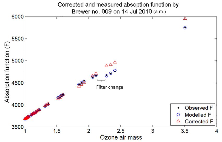
Z. Vaziri Zanjani et al.: A non-linearity calibration for Brewer 275
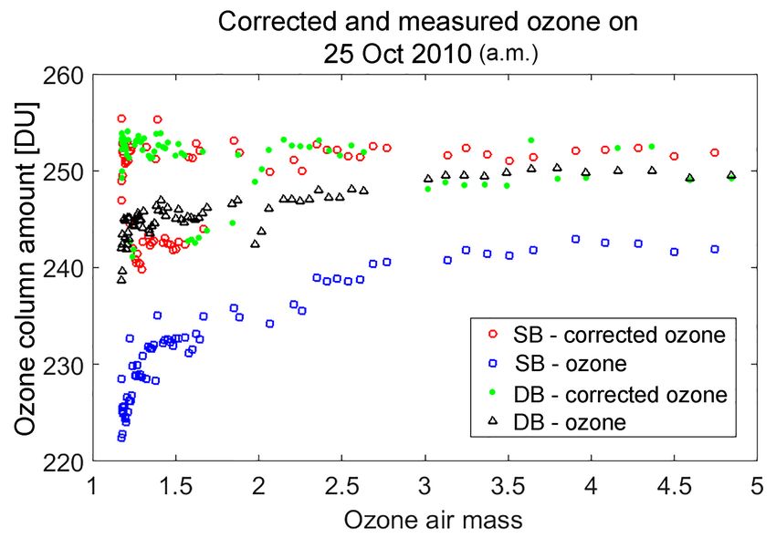
Figure 4. Observed, modelled and corrected absorption function
(F ) for double Brewer no. 119. The corrected values are very close Figure 5. Corrected and measured ozone by single (SB no. 009)
to observed due to the double Brewer’s ability to reject stray light and double (DB no. 119) Brewer on 14 July 2010.
better than the single Brewer.
and high-intensity solar radiation, a small change of 10 ns in
the dead time can cause an error of up to 5 % in the measured
total ozone column amount (Fountoulakis et al., 2016). The
dead-time correction is modelled in Eq. (15) where N is the
measured photon count, N0 is the corrected photon count and
τ is the dead time (Kerr, 2010).
N = N0 · eN0 ·τ (15)
To calculate dead time, measurements are done with the
Brewer through two exit slits simultaneously and separately
through each exit slit. For example, measurements are done
with exit slit 2 and 4 resulting in N2 and N4 and measure-
ments are done with both exit slits open resulting in N2+4 .
If Eq. (15) is written for each case, three equations with four Figure 6. Ratio of measured and corrected single (SB) to double
unknowns result, which are N02 , N04 , N02+4 and τ . A fourth Brewer (DB) ozone values for data points measured within 5 min of
equation, N02+4 = N02 + N04 , will help find the dead time each other on 14 July 2010.
(Kerr, 2010). This procedure is not done on a regular basis
and the dead time of an instrument changes somewhat over
time; therefore a correction prediction for dead time must be 3 Results and discussion
performed during the Langley process. To account for the
dead-time prediction, when calculating the derivative of the The Langley method was applied to the data collected by
square error, SE, the derivative of Fi with respect to dead two Brewer instruments no. 009 (single Brewer) and no. 119
time must also be considered. In this case, vk is τ and thus (double Brewer) stationed at Mauna Loa at −155.5◦ longi-
Eq. (8) becomes Eq. (16), which shows how this derivative is tude and 19.5◦ latitude, and as an example the results for
included in the Langley method. 14 July and 25 October 2010 are presented. The non-linear
mathematical model (Eq. 5) was applied to the data and
∂ (Fi ) model parameters where retrieved. The non-linearity term,
Mik = − (16)
∂τ filter change term and dead-time term were applied in reverse
to the data to calculate corrected values for the absorption
function and ozone values in Dobson units.
The observed, modelled and corrected absorption function
(F ) for single Brewer no. 009 is plotted in Fig. 3. In the ob-
served and modelled F , you can clearly see the filter change
causing a jump in the intensity of light received by the de-
tector. This sudden fluctuation in intensity is modelled using
www.atmos-meas-tech.net/12/271/2019/ Atmos. Meas. Tech., 12, 271–279, 2019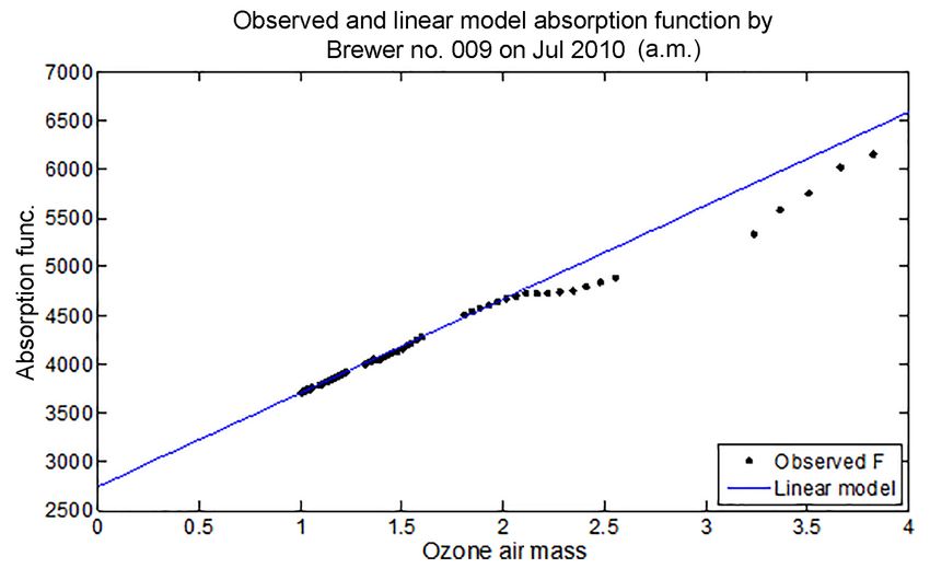
276 Z. Vaziri Zanjani et al.: A non-linearity calibration for Brewer
Table 1. Standard ozone retrieval parameters compared to parameters retrieved from the model (14 July 2010).
Single no. 009 Double no. 119
Ozone retrieval parameters
Standard Model Standard Model
Extraterrestrial constant (ETC) 2855 2783.8 1647 1639.3
Dead time (DT) 3.9 × 10⁻⁸ 3.27502 × 10⁻⁹ 4.2 × 10⁻⁸ 1.6 × 10⁻⁹
Non-linearity factor (γ ) – 7.8 × 10⁻¹⁷ – 2.7 × 10⁻¹⁷
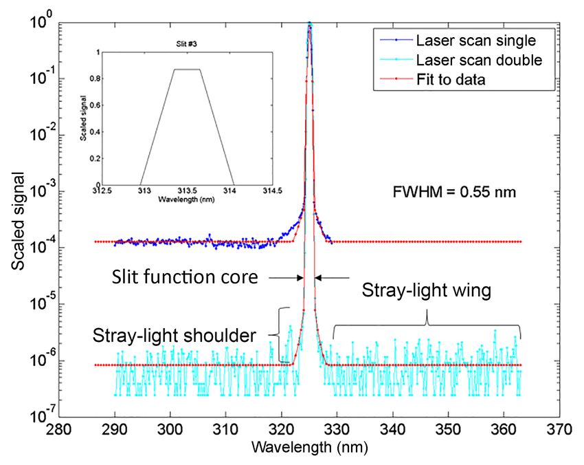
Figure 7. Corrected and measured ozone by single (SB no. 009) Figure 8. Ratio of measured and corrected single (SB) to double
and double (DB no. 119) Brewer on 25 October 2010. Brewer (DB) ozone values for data points measured within 5 min of
each other on 25 October 2010.
the non-linear model and is corrected to give a more linear
F with respect to ozone air mass. The same has been plotted 4 Conclusions
for the double Brewer no. 119 in Fig. 4, where the observed
modelled and corrected observations are very close to linear There is a difference of up to 10 % in the ozone column
with respect to air mass, and thus the correction is less than amount measured by the single and double Brewers (single
1 %. lower than double) as observed at large ozone slant paths and
Using the corrected absorption function, the corrected illustrated in Fig. 5 for 14 July 2010 and Fig. 7 for 25 Octo-
ozone values were calculated. The measured and corrected ber 2010. The mathematical model presented in this paper
ozone column amounts in Dobson units vs. ozone air mass accounts for this non-linearity in the data collected by single
for both the single (no. 009) and double (no. 119) Brewers Brewers. Applying corrections to the historical data of sin-
for 14 July and 25 October 2010 are illustrated in Figs. 5 gle Brewers is essential, as it will eliminate errors due to the
and 7 respectively. There is some non-linearity observed effect of stray light in the ozone measurements.
for the single Brewer at low air mass which is corrected to The double Brewer more accurately rejects stray-light ef-
an amount slightly higher than the double Brewer-corrected fects (Gröbner et al., 1998), and as the single Brewers in
amounts. The ratios of single to double Brewer measure- ozone measurement stations around the world are being re-
ments before and after applying corrections for 14 July and placed by the more advanced double Brewer, a slight increase
25 October 2010 are plotted in Figs. 6 and 8 respectively. in the ozone amounts may be observed, particularly in those
The corrected ratio in red is closer to linearity than the un- months in which observations must necessarily be made at
corrected ratio in black. As a comparison the obtained pa- large solar zenith angles. This may lead to a false assumption
rameters from the model and the standard parameters used to that the total ozone column amounts are showing an increas-
retrieve ozone for 14 July 2010 can be seen in Table 1. ing trend when this may not be the case.
The departure from linearity is more prominent for large
air mass (µ) values as is seen in Figs. 3, 5 and 7. This
non-linearity at large air masses becomes more prominent in
high-latitude regions such as the Arctic, where the sun is at
large solar zenith angles most of the year. It is also difficult
Atmos. Meas. Tech., 12, 271–279, 2019 www.atmos-meas-tech.net/12/271/2019/Z. Vaziri Zanjani et al.: A non-linearity calibration for Brewer 277
to take reference Brewer instruments to the Arctic for cal-
ibration purposes. To provide an accurate on-site method to
correct the ozone data for non-linearity, the process described
in this paper is recommended.
The future steps for this research will be to apply this
method to historical databases and produce an applicable
software that would output corrected daily ozone values.
Data processing using the new methodology leads to a more
accurate absolute calibration on single Brewers and to a way
to properly transfer calibration constants between single and
double Brewers.
Data availability. Data available at
– https://doi.org/10.5281/zenodo.2531911 (Vaziri Zanjani,
2019a),
– https://doi.org/10.5281/zenodo.2531905 (Vaziri Zanjani,
2019b),
– https://doi.org/10.5281/zenodo.2531955 (Vaziri Zanjani,
2019c) and
– https://doi.org/10.5281/zenodo.2531951 (Vaziri Zanjani,
2019d).
www.atmos-meas-tech.net/12/271/2019/ Atmos. Meas. Tech., 12, 271–279, 2019278 Z. Vaziri Zanjani et al.: A non-linearity calibration for Brewer
Appendix A: Jacobian calculations of Mik :
∂ (Fmi )
Mik =
∂vk
∂ (Fmi )
Mi1 = = −α · µ − 3γ · (α · µ)3 · (x)2
∂x
∂ (Fmi )
Mi2 = = −(α · µ · x)3
∂γ
∂ (Fmi )
Mi3 = = NDj
∂bj
∂ (Fmi )
Mi4 = =1
∂F0
∂ (Fmi )
Mi5 = = −104 · w · Cλ
∂τ
Atmos. Meas. Tech., 12, 271–279, 2019 www.atmos-meas-tech.net/12/271/2019/Z. Vaziri Zanjani et al.: A non-linearity calibration for Brewer 279
Author contributions. ZVZ contributed by developing the mathe- Moeini, O., Vaziri, Z., McElroy, C. T., Tarasick, D. W., Evans, R. D.,
matical model and MATLAB software to analyze and correct for Petropavlovskikh, I., and Feng, K.-H.: The Effect of Instrumental
the non-linearity caused by stray light present in the ozone mea- Stray Light on Brewer and Dobson Total Ozone Measurements,
surements by the Brewer instrument. OM developed the physical Atmos. Meas. Tech. Discuss., https://doi.org/10.5194/amt-2018-
model of the Brewer instrument. TME, DB and VS assisted in writ- 2, in review, 2018.
ing the paper and provided valuable discussions about the Brewer Redondas, A., Evans, R., Stuebi, R., Köhler, U., and We-
retrievals and measurements. ber, M.: Evaluation of the use of five laboratory-determined
ozone absorption cross sections in Brewer and Dobson re-
trieval algorithms, Atmos. Chem. Phys., 14, 1635–1648,
Competing interests. The authors declare that they have no conflict https://doi.org/10.5194/acp-14-1635-2014, 2014.
of interest. Redondas, A., Carreño, V., León-Luis, S. F., Hernández-Cruz,
B., López-Solano, J., Rodriguez-Franco, J. J., Vilaplana, J. M.,
Edited by: Andreas Hofzumahaus Gröbner, J., Rimmer, J., Bais, A. F., Savastiouk, V., Moreta,
Reviewed by: three anonymous referees J. R., Boulkelia, L., Jepsen, N., Wilson, K. M., Shirotov, V.,
and Karppinen, T.: EUBREWNET RBCC-E Huelva 2015 Ozone
Brewer Intercomparison, Atmos. Chem. Phys., 18, 9441–9455,
https://doi.org/10.5194/acp-18-9441-2018, 2018.
References Rimmer, J. S., Redondas, A., and Karppinen, T.: EuBrewNet
– A European Brewer network (COST Action ES1207),
Bais, A. F., Zerefos, C. S., and McElroy, C. T.: Solar UVB mea- an overview, Atmos. Chem. Phys., 18, 10347–10353,
surements with the double- and single-monochromator Brewer https://doi.org/10.5194/acp-18-10347-2018, 2018.
ozone spectrophotometers, Geophys. Res. Lett., 23, 833–836, Savastiouk, V.: Improvements To the Direct-Sun Ozone Observa-
https://doi.org/10.1029/96GL00842, 1996. tions Taken With the Brewer Spectrophotometer, York Univer-
Fioletov, V. E., Kerr, J. B., Wardle, D. I., and Wu, E.: Correction of sity, available at: https://www.esrl.noaa.gov/gmd/grad/neubrew/
stray light for the Brewer single monochromator, Proc. Quadren- docs/publications/VladimirSavastiouk_PhD_thesis.pdf (last ac-
nial Ozone Symposium, 21, 369–370, 2000. cess: 2018), 2006.
Fountoulakis, I., Redondas, A., Bais, A. F., Rodriguez-Franco, J. J., Savastiouk, V. and McElroy, C. T.: Brewer spectrophotometer to-
Fragkos, K., and Cede, A.: Dead time effect on the Brewer mea- tal ozone measurements made during the 1998 Middle Atmo-
surements: correction and estimated uncertainties, Atmos. Meas. sphere Nitrogen Trend Assessment (MANTRA) Campaign, At-
Tech., 9, 1799–1816, https://doi.org/10.5194/amt-9-1799-2016, mos. Ocean, 43, 315–324, https://doi.org/10.3137/ao.430403,
2016. 2005.
Gröbner, J., Wardle, D. I., McElroy, C. T., and Kerr, J. B.: Investi- Silva, A. A. and Kirchhoff, V. W. J. H.: Aerosol optical thickness
gation of the wavelength accuracy of brewer spectrophotometers, from Brewer spectrophotometers and an investigation into the
Appl. Optics, 37, 8352–8360, 1998. stray-light effect, Appl. Optics, 43, 2484–2489, 2004.
Josefsson, W. A. P.: Focused Sun Observations Using a Brewer Slavin, W.: Stray Light in Ultraviolet, Visible and Near-Infrared
Ozone Spectrophotometer, J. Geophys. Res., 97, 15813–15817, Spectrophotometry, Anal. Chem., 35, 561–566, 1963.
1992. Vaziri Zanjani, Z.: Brewer 009_25 Oct 2010 [Data set], Zenodo,
Karppinen, T., Redondas, A., García, R. D., Lakkala, K., https://doi.org/10.5281/zenodo.2531911, 2019a.
McElroy, C. T., and Kyrö, E. Compensating for the ef- Vaziri Zanjani, Z.: Brewer 009_14 Jul 2010 [Data set], Zenodo,
fects of stray light in single-monochromator brewer spec- https://doi.org/10.5281/zenodo.2531905, 2019b.
trophotometer ozone retrieval, Atmos. Ocean, 53, 66–73, Vaziri Zanjani, Z.: Brewer 119_14 Jul 2010_AM,
https://doi.org/10.1080/07055900.2013.871499, 2015. https://doi.org/10.5281/zenodo.2531955, 2019c.
Kerr, J. B.: The Brewer Spectrophotometer, in: UV Radiation in Vaziri Zanjani, Z.: Brewer 119_ 25 Oct 2010_ AM [Data set], Zen-
Global Climate Change, edited by: Gao, W., Schmoldt, D. L., and odo, https://doi.org/10.5281/zenodo.2531951, 2019d.
Slusser, J. R., Tsinghua University Press, Beijing and Springer, WOUDC: instrument list is available at: http://www.woudc.org/
160–191, 2010. data/instruments/ (last access: 1 May 2017), 2016.
Kerr, J. B., McElroy, C. T., Wardle, D. I., Olafson, R. A., and Evans,
W. F. J. The automated Brewer spectrophotometer, in: Quadren-
nial Ozone Symposium, edited by: Zerefos, C. S. and Ghazi, A.,
Halkidiki, Greece, 396–401, 1984.
www.atmos-meas-tech.net/12/271/2019/ Atmos. Meas. Tech., 12, 271–279, 2019You can also read