Global Mercury Footprint Evaluation using a Geographical Pollutant Propagation Model - aidic

1213

 A publication of

 CHEMICAL ENGINEERING TRANSACTIONS
VOL. 81, 2020 The Italian Association
 of Chemical Engineering
 Online at www.cetjournal.it

Guest Editors: Petar S. Varbanov, Qiuwang Wang, Min Zeng, Panos Seferlis, Ting Ma, Jiří J. Klemeš
Copyright © 2020, AIDIC Servizi S.r.l.
 DOI: 10.3303/CET2081203
ISBN 978-88-95608-79-2; ISSN 2283-9216

 Global Mercury Footprint Evaluation using a Geographical
 Pollutant Propagation Model
Anna Makarovaa,*, Ravil Yakubovb, Petar Sabev Varbanovс
a
 UNESCO Chair ‘Green Chemistry for Sustainable Development’, Mendeleev University of Chemical Technology of Russia,
 125047 Miusskaya sq. 9, Russian Federation
b
 Department of Logistics and Economic Informatics, Mendeleev University of Chemical Technology of Russia, 125047
 Miusskaya sq. 9, Russian Federation
c
 Sustainable Process Integration Laboratory – SPIL, NETME Centre, Faculty of Mechanical Engineering, Brno University of
 Technology - VUT Brno, Technická 2896/2, 616 69 Brno, Czech Republic
 annmakarova@muctr.ru

This work presents a method for the accurate evaluation of the footprint of chemical pollutants on a global scale.
An extension of the standard pollution propagation models is proposed to calculate the chemical footprint
efficiently. The proposed improvements overcome the current modelling and enable the evaluation of the
directed transport of chemicals with water or air flows. The current research introduces several model
modifications to account for the directed pollutant transport with global water flows and selects the Jacobi
solution method for the resulting large-scale system of mass transfer equations. The model was combined with
geographic information system data to account for the geographical propagation of the pollutants. The proposed
method is implemented in Microsoft Excel using the built-in Visual Basic for Applications programming language.
The method is tested on the example of evaluating the Global Mercury Footprint. As a result of the work, a tool
was obtained that allows estimating the chemical load for the entire World, taking into account the transfer of
chemicals with water flows. In the future, this tool can also be used to support regulatory decisions, for example,
to assess the effect of mercury immobilization in solid waste on the mercury footprint.

1. Introduction
Prediction of the environmental impact of anthropogenic chemicals is a critical component of decision-making
when choosing chemicals for use in production and everyday life. This is especially important when assessing
the potential risks to human health and the environment when introducing new products/substances. Chemical
load modelling is one of the main forecasting tools. In particular, an acute example of a chemical component in
need of a global and accurate evaluation is mercury. This has been widely recognized by the scientific
community, as can be witnessed by the review of mercury emissions from energy generation (Charvát et al.,
2020). This is a global pollutant (Tauqeer et al., 2015). By 2020, according to the provisions of the Minamata
Convention on Mercury (IPEN, 2018), the countries that have ratified the Convention, must phase out mercury-
containing products: batteries, switches and relays, mercury lamps, thermometers etc. It should be noted that
according to Tarasova et al. (2018), such products and their waste are among the most significant sources of
mercury pollution (UN Environment, 2017). Takaoka (2015) confirms this for the case of Japan. Mercury can
also be released from the incineration of mercury-containing household waste, such as e-waste, medical waste,
and consumer products (compact fluorescent lamps, cosmetics, switches, thermometers) (IPEN, 2018). It has
been estimated that up to 10 % of the current anthropogenic mercury emissions are released by open burning
of such waste materials (Wiedinmyer et al., 2014). The global inventory of atmospheric mercury emissions from
anthropogenic sources amounts to 2,000 - 3,000 t/y. Mercury emissions associated with the disposal of mercury-
added product waste is 7 % of this (UN Environment, 2019).
Models describing the behavior (including transformation) of chemicals and their propagation into various natural
media have been developed. Such are the models CalTOX (2020) – updated but not actively developed, BETR
(2020) – partitioning the World map into 15 ° cells, USEtox (2020) – referred to as the “scientific consensus

Paper Received: 17/05/2020; Revised: 26/06/2020; Accepted: 30/06/2020
Please cite this article as: Makarova A., Yakubov R., Varbanov P.S., 2020, Global Mercury Footprint Evaluation using a Geographical Pollutant
Propagation Model, Chemical Engineering Transactions, 81, 1213-1218 DOI:10.3303/CET2081203

1214

model”, with its implementation (MacLeon et al., 2005). Of these, the USEtox model has several advantages.
One is the database containing information on the ecotoxicological characteristics of approximately 2,500
chemicals – including mercury and other heavy metals (Rosenbaum et al., 2008). In the standard USEtox model,
natural media are represented as compartments that contain a pollutant.
The environment is described in the USEtox model (Figure 1) in the form of a 2-tier system comprising regional
and global levels, each of which includes compartments describing atmospheric air (urban and rural),
agricultural soil, and soils of other types, freshwater, and coastal seawater or ocean. Depending on the
processes taking place in a compartment, the pollutant may remain within the chamber where it was initially
released, may be transformed into other chemicals via, e.g., hydrolysis or oxidation, or may migrate to another
compartment (Fantke et al., 2017).

Figure 1: The model of mass transfer between cells (S - sources of hazardous chemicals, k - rate constants for
the transfer/degradation/removed of chemicals)

Another model is Pangea (2020), developed by Australian scientists in 2017. It has been designed to estimate
the content of chemicals in water, soil, and air, taking into account their propagation with water flows (Wannaz
et al., 2018). The environmental process models in Pangea are currently based on the IMPACT (Pennington et
al., 2005) and USEtox models, adapted for taking spatial data into account, aided by the use of Geographic
Information Systems. The mode is of hierarchical nature, containing several levels. It lumps cells with similar
properties into more massive clusters. This modelling technique greatly simplifies the solution but also leads to
loss of accuracy and fidelity due to the lumping the measurement errors.
An alternative way of solving the large-scale matrix of mass balances is to use the original maps, avoiding data
aggregation. The standard USEtox model was used as the basis for formulating the mass transfer equations,
which is constitute the central part of the model for chemical footprint analysis. To take into account the transfer
of chemicals with water flows, the USEtox model was adapted (Makarova et al., 2018). Instead of one local level
as in the USEtox model, that work introduced a set of local levels (cells) (Figure 1). That allowed the model to
take into account the interaction between the local levels, e.g., directed transfer of chemicals with water or air
flows. The model was combined with GIS (Geographical Information System) data to solve this task, partitioning
the studied area for the entire World on a 0.5 ° by 0.5 ° grid. In the model construction, the ocean and the
atmospheric air above it remain at the global level. However, unlike the Pangea model, the cell scale was not
enlarged. Instead, the model used the scale of the GIS data directly, avoiding additional interference to the initial
data due to lumping. This chemical footprint model of the entire World results in a very large-scale underlying
matrix of mass balance equations – of the size 1.5×106 (equations × variables) (Makarova et al., 2019).
In summary, the two main approaches to modelling the transfer and propagation of chemicals for estimating
their impacts and footprints, resort to either highly lumped models or to the use of a finer map mesh. The issue
with the lumped models lies in the amplification of the inaccuracies of the processed data, to the point that the
model may be no longer representative of the problem. On the other hand, the finer-grained models result in a
very large-scale matrix of equations, which takes an extremely long time to solve or does not converge at all.
The current paper presents an approach to solving the natural-scale system of equations in a reasonable time

1215

and with the desired accuracy. The proposed method solves the equations of the USETox model in the variant
of one global level and many local ones. The novel element is the introduction of additional degrees of freedom
in the model, which allows accounting also for the mass transfer between the model compartments for air and
ocean. The resulting system of equations is solved directly using the original GIS data on maps of 0.5 to 0.5
degrees without introducing intermediate aggregated levels and, without averaging the original GIS data, and
without the errors associated with this averaging.

2. Evaluation method and computational results
The chemicals in the cell mainly come from stationary technogenic sources (Sp,n = const (kg/s)). Assuming
steady-state conditions, the following system of equations is obtained for the cells n = (1, N):
 6 6

 , = ∑ ∑ , → , , , − ∑ ∑ , → , , + , , , + , , , (1)
 =1 =1 =1 =1

Where: n, i = {a, as, ns, sw, ua, w} compartments in a cell denoting natural media; j,p = {1.. 259, 200}: cells on
the map; Sp,n – chemical intake flow in the current compartment n in cell p (kg/s); mp,n – the mass of the chemical
in the current compartment n in cell p (kg); mi,j – the mass of the chemical in the compartment i in cell j (kg).
The model expressed in Eq(1) takes as specifications:
• The migration rate kp,n→i,j (s-1) - between compartment n of the cell p and compartment i of the cell j, denoted
 as ka-wj (s-1) in Figure 1 for the case of mass transfer from rural air of the cellj to the freshwater of the cellj;
• The degradation rate kdeg,p,n (s-1) compartment n of the cell p, - denoted as kdeg.wj (s-1) in Figure 1 for the case
 of the chemical degradation in freshwater in cellj;
• The rate of removal ksed,n (s-1) from cell p to sediment - denoted as kw-sed,j (s-1) in Figure 1 in case cellj.
In Eq(1), the terms have the following meaning:
• kp,n→i,jmp,n – migration rate of the chemical from compartment n of cell p to compartment I, cell j (kg/s);
• ki,j→p,nmi,j – migration rate of the chemical from compartment i of cell j to compartment n of cell p (kg/s);
• kdeg,p,nmp,n – degradation rate of the chemical in the investigated compartment n of the cell p (kg/s);
• ksed,nmp,n – chemical removal rate in sediments in the investigated compartment n of the cell p (kg/s).
An additional modelling element proposed in this study, at the stage of compiling the matrix of transfer
coefficients, is to take into account the mass exchanges between the compartments for global air and the ocean
due to the chemicals transfer. In a previous work (Makarova et al., 2019), which did not account for mass
contaminant transfer concerning the ocean and atmospheric air components, this system of linear equations
could not be solved by iterative methods.
Specifying more accurate values for the migration coefficients in global air and the ocean makes it possible to
successfully use both direct and iterative methods for solving the system of contaminant mass balances.
The following approaches (Saad, 2007) to solve the model have been tested: Bistabilized Gradient Method,
Linear Solver restarted GMRES (Generalised Minimum RESidual) and the MINRES (MINimum RESidual)
iteration methods, the Jacobi method, the LGMRES method with a preconditioner – all supplied with the Python
library (SciPy, 2020),
The first method evaluated for solving the model was the Bistabilized Gradient Method, in which initial guess mn
= 0 kg/s was taken. This method showed low efficiency, and after more than 10,000 iterations (Figure 2), no
convergence was achieved. The merging was estimated using the residual norm equal to the square root of the
sum of the squared deviations.

 1×108
 100,000,000
 Logarithmic scale
 Residual norm (1)

 1×107
 1,000,0006
 1×10
 1×105
 10,000
 1×104
 1×103
 100
 100
 1
 10
 0 2,000 4,000 6,000 8,000 10,000 12,000 14,000 16,000
 1
 Iteration

Figure 2: The residual norm for the Bistabilised Gradient Method

1216

The next to solve this system were the iterative methods LGMRES (Linear Solver restarted GMRES), MINRES
(MINimum RESidual iteration) and LSMR (Iterative solver for least-squares problems) (SciPy, 2020) from the
linear algebra module for sparse matrices (scipy.sparse.linalg) in Python Figure 3a shows the dependence of
the residual norm for the LGMRES method. The residual norm starts from 137 (1) and stabilises at 55.7 (1).
When solving using the MINRES method (Figure 3b), the residual norm also starts from 137 (1). and then
stabilises at 20.4 (1). These results are better, but the achieved convergence was poor.
 140 b)
 a)

 Residual norm (1)
 140 120
 120
 Residual norm (1)

 100
 100 80
 80
 60
 60
 40
 40
 20 20
 0 0
 0 2,000 4,000 6,000 8,000 10,000 0 500 1,000 1,500 2,000 2,500
 Iterations Iterations

Figure 3: The residual norm in linear scale: a) for the LGMRES method, b) for the MINRES method

The Jacobi method, which previously worked only on a partitioned matrix, after the proposed model changes,
converges relatively quickly for 394 (1) to a solution with an accuracy of 9.8×10-10 (1), demonstrating excellent
final convergence. The graph of the error in the usual and logarithmic coordinates is presented in Figure 4.

 1×104 Logarithmic scale 5,000
 Residual norm (1)

 1×102
 1E+02 Linear scale
 Residual norm (1)

 4,000
 1E-011
 1×10-2 3,000
 1E-04-4
 1×10 2,000
 1E-07-6
 1×10 1,000
 1×10-8
 1E-10 0
 106
 127
 148
 169
 190
 211
 232
 253
 274
 295
 316
 337
 358
 379
 1

 85
 22
 43
 64
 1

 106

 253
 127
 148
 169
 190
 211
 232

 274
 295
 316
 337
 358
 379
 22
 43
 64
 85

 Iterations Iterations

Figure 4: The residual norm for the Jacobi method in logarithmic and linear scale

The solution of the System of Linear Algebraic Equations using the LGMRES method with a preconditioner was
also considered. The preconditioner was obtained using the scipy.sparse.linalg.spilu function (based on the
Supernodal sparse direct solver). This resulted in a significant convergence acceleration. The sufficiently low
residual norm at 6×10-10 (1) was already at the 3-rd iteration (Figure 5).

 1×104
 1E+04
 Residual norm (1)

 1E+02
 1×102
 1E+001
 1E-02
 1×10-2
 1E-04
 1×10 -4
 1E-06
 1E-08-6
 1×10
 1E-10-8
 1×10
 1E-12
 1×10 -10
 1E-14
 1×10 -12
 0 2 4 6 8 10
 1×10-14
 Iterations

Figure 5: The residual norm for the LGMRES method with a preconditioner in logarithmic scale

For all considered iterative methods, a vector consisting of only 0 was taken as the initial approximation of the
solution. Using the direct solution method spsolve from the scipy.sparse.linalg module (based on the
UMFPACK package), it was possible to obtain a solution with a residual norm of 6.48×10-10 (1).
For quantifying the Global Mercury Footprint, the proposed model uses data on mercury emissions from
anthropogenic sources. They were taken from the Arctic Monitoring and Assessment Program (AMAP/UNEP,
2013), which provides datasets on a 0.5 ° x 0.5 ° grid. These include emissions in kg/”grid cell”, and the grid cell

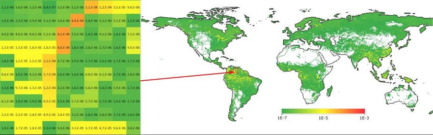
1217

area (km2). The 2010 global mercury intake flows (Sp,n in Eq(1)) into the atmosphere, coming from anthropogenic
sources, were determined for:(a) Stationary combustion sources: power plants, distributed heating, and energy
use (excluding industry); (b) Industrial sources; (c) Sectors related to intentional use and product waste.

3. Analysis and discussion
The case study model has been solved using the Jacobi method as the best-performing one. This method, as
also the LGMRES method with a precondition, allows us to quickly find a solution (Figure 4) tor the created
matrix. However, the Jacobi method, unlike the LGMRES method with a precondition, is much simpler to
implement and does not require additional software. The Jacobi method produced six maps of Global Mercury
Footprint by environmental compartments – urban air, rural air, freshwater, seawater, agricultural soil, other soil.
Figure 6 shows the Mercury Footprint for freshwater bodies calculated by the proposed model. The green color
indicates areas in which the mercury concentration lower than the maximum permissible for the fishery. Yellow
denotes areas where the maximum concentration limit for drinking water is exceeded (moderate heath risk),
and red indicates extremely high levels posing a very serious danger to humans and biota. The map clearly
shows the spread of mercury contamination in highly populated regions or regions of sourcing food, indicating
the high level of threat to human health. These results correlate very much with the measured data of mercury
concentrations in aquatic species (Evers et al., 2018), as well as with a map of global mercury-related worker
disability (Steckling et al., 2017).

Figure 6: Mercury footprint for freshwater bodies calculated by the proposed model

4. Conclusions
The current work presents a model extension and a solution method for the evaluation of Global Chemical
Footprints. Its efficiency and achievable accuracy have been demonstrated on the example of Global Mercury
Footprint evaluation. The Jacobi method proved as the most efficient in obtaining the solution in several hundred
iterations, compared with the slow convergence or the lack of that in previous chemical footprint evaluation
models. The achieved convergence can be characterised quantitatively by the reduction of the residual norm
from the order of 103 down to 10-10. The results confirm the ability of the proposed model to evaluate the chemical
footprints of any pollutants subject to data availability. The produced maps of Global Mercury Footprint provide
better accuracy than the general maps lumping deceases by countries. The current model can be further
extended to include a modelling component accounting for atmospheric transport of the pollutants, which
presents an excellent avenue for future research.

Acknowledgements
The current research has been funded by the RFBR according to the research project № 18-29-24212 and by
the EU supported project Sustainable Process Integration Laboratory – SPIL funded as project No.
CZ.02.1.01/0.0/0.0/15_003/0000456, by Czech Republic Operational Programme Research and Development,
Education, Priority 1: Strengthening capacity for quality research.

References
AMAP/UNEP, 2013, AMAP/UNEP geospatially distributed mercury emissions dataset 2010v1,
 , accessed 20.04.2020.

1218

BETR Global, 2020, Geographically Explicit Global-Scale Multimedia Contaminant Fate Model,
 , accessed 10.02.2020.
CalTox, 2020, The Department of Toxic Substances Control, CA, USA, , accessed 04.06.2020.
Charvát P., Klimeš L., Pospíšil J., Klemeš J.J., Varbanov PS, 2020, An overview of mercury emissions in the
 energy industry - A step to mercury footprint assessment, Journal of Cleaner Production, 267, 122087.
IPEN, 2018. Mercury emissions from the open burning of waste. IPEN combined submission to the Minamata
 Convention secretariat on 26/08/2018 , accessed 25.02.2020.
Evers D.C., Taylor M., Burton M., Johnson S., 2018, Mercury in the Global Environment: Understanding spatial
 patterns for biomonitoring needs of the Minamata Convention on Mercury. Biodiversity Research Institute.
 Portland, Maine. BRI Science Communications Series 2018-21. 21 pages.
 , accessed 14.05.2020.
Fantke P. (Ed), 2017, USEtox®2.0 Documentation - International Center hosted at the Technical University of
 Denmark, Copenhagen, Denmark.
MacLeod M., Riley W. J., McKone T. E., 2005, Assessing the influence of climate variability on atmospheric
 concentrations of polychlorinated biphenyls using a global624 scale mass balance model (BETR-Global).
 Environ. Sci. Technol. 39 (17), 6749–6756.
Makarova A., Shlyakhov P., Tarasova N., 2018, Estimating chemical footprint on high-resolution geospatial grid.
 Procedia CIRP 69, 469–474, DOI: 10.1016/j.procir.2018.01.001.
Makarova A., Fedoseev A., Pischaeva K., 2019, Assessment of the mercury footprint at the global scale. In:
 Book of abstracts 14th Conference on Sustainable Development of Energy, Water and Environment Systems
 (SDEWES), Dubrovnik, Croatia, paper SDEWES19.217.
Pangea, 2020, The Pangea Model, , accessed 10.02.2020.
Pennington D.W., Margni M., Ammann C., Jolliet O., 2005, Multimedia fate and human intake modeling: Spatial
 versus nonspatial insights for chemical emissions in Western Europe. Environ. Sci. Technol., 39(4), 1119–
 1128.
Rosenbaum R.K., Bachmann T.M., Gold L.S., Huijbregts M.A.J., Jolliet O., Juraske R., Koehler A., Larsen H.F.,
 MacLeod M., Margni M., McKone T.E., Payet J., Schuhmacher M., Van de Meent D., Hauschild M.Z., 2008,
 USEtox — the UNEP-SETAC toxicity model: recommended characterisation factors for human toxicity and
 freshwater ecotoxicity in life cycle impact assessment. International Journal of Life Cycle Assessment, 13(7),
 532–546, DOI 10.1007/s11367-008-0038-4.
Saad Y., 2003, Iterative Methods for Sparse Linear Systems (2nd Ed.). SIAM, Philadelphia, USA. ISBN 978-0-
 89871-534-7.
SciPy, 2020, SciPy — SciPy v1.4.1 Reference Guide, , accessed 5.5.20.
Steckling N., Tobollik M., Plass D., Hornberg C., Ericson B., Fuller R., Bose-O’Reilly S., 2017. Global Burden of
 Disease of Mercury Used in Artisanal Small-Scale Gold Mining. Annals of Global Health, Current Topics in
 Global Health, 83, 234–247.
Takaoka M., 2015, Mercury and mercury-containing waste management in Japan. Journal of Material Cycles
 and Waste Management, 17(4), 665-672, DOI:10.1007/s10163-014-0325-z.
Tarasova NP, Makarova A.S., Vinokurov S.F., Kuznetsov V.A., Shlyakhov P.I., 2018, Green chemistry and
 sustainable development: approaches to chemical footprint analysis. Pure Appl. Chem., 90(1), 143-155,
 DOI:10.1515/pac-2017-0608.
Tauqeer A., Nazir S., Overgard K., Manca D., Mutaliba M., Khan E., 2015, Hazards of Mercury – Safety
 Perspectives and Measures. Chemical Engineering Transactions, 43, 2143-2148, DOI:
 10.3303/CET1543358.
UN Environment, 2017, Global mercury supply, trade and demand. United Nations Environment Programme,
 Chemicals and Health Branch. Geneva, Switzerland.
UN Environment, 2019, Global Mercury Assessment, 2018, UN Environment Programme, Chemicals and
 Health Branch, Geneva, Switzerland. ISBN: 978-92-807-3744-8.
USEtox, 2020, Scientific Consensus Model, , accessed 10.02.2020.
Wiedinmyer C., Yokelson R., Gullett B., 2014, Global Emissions of Trace Gases, Particulate Matter, and
 Hazardous Air Pollutants from Open Burning of Domestic Waste. Environ. Sci. Technol. 48 (16), 9523−9530.
 DOI:10.1021/es502250z.
Wannaz C., Fantke P., Lane J., Jolliet O., 2018, Source-to-exposure assessment with the Pangea multi-scale
 framework – case study in Australia, Environ Sci Process Impacts, 20(1), 133-144, DOI:
 10.1039/c7em00523g.