Trapezoid-grid finite difference frequency domain method for seismic wave simulation

Journal of Geophysics and Engineering
Journal of Geophysics and Engineering (2021) 18, 594–604 https://doi.org/10.1093/jge/gxab038

Trapezoid-grid finite difference frequency domain
method for seismic wave simulation
Bangyu Wu1 , Wenzhuo Tan1 and Wenhao Xu2,*
1
 School of Mathematics and Statistics, Xi’an Jiaotong University, Xi’an, Shaanxi Province 710049, China

 Downloaded from https://academic.oup.com/jge/article/18/4/594/6350127 by guest on 19 October 2021
2
 School of Information and Communications Engineering, Xi’an Jiaotong University, Xi’an, Shaanxi Province
710049, China

*Corresponding author: Wenhao Xu. E-mail: doumifeiniao@163.com

Received 10 May 2021, revised 6 July 2021
Accepted for publication 16 July 2021

Abstract
The large computational cost and memory requirement for the finite difference frequency
domain (FDFD) method limit its applications in seismic wave simulation, especially for large
models. For conventional FDFD methods, the discretisation based on minimum model velocity
leads to oversampling in high-velocity regions. To reduce the oversampling of the conventional
FDFD method, we propose a trapezoid-grid FDFD scheme to improve the efficiency of wave
modeling. To alleviate the difficulty of processing irregular grids, we transform trapezoid grids in
the Cartesian coordinate system to square grids in the trapezoid coordinate system. The regular
grid sizes in the trapezoid coordinate system correspond to physical grid sizes increasing with
depth, which is consistent with the increasing trend of seismic velocity. We derive the trapezoid
coordinate system Helmholtz equation and the corresponding absorbing boundary condition,
then get the FDFD stencil by combining the central difference method and the
average-derivative method (ADM). Dispersion analysis indicates that our method can satisfy the
requirement of maximum phase velocity error less than 1% with appropriate parameters.
Numerical tests on the Marmousi model show that, compared with the regular-grid ADM
9-point FDFD scheme, our method can achieve about 80% computation efficiency improvement
and 80% memory reduction for comparable accuracy.
Keywords: frequency domain, finite difference, trapezoid-grid method, seismic wave modeling

1 Introduction of simulation and reduce the bandwidth of the impedance
 matrix, many studies of the FDFD method focus on how
In order to achieve more efficient seismic migration (Herman
 to decrease the required number of points per wavelength
et al. 1982; Chung et al. 2011; Shi et al. 2019; Liu et al. 2021)
 (NPPW) while using fewer grid points in the FDFD scheme
and inversion (Yang et al. 2018; Hu et al. 2019; da Costa
 ( Jo et al. 1996; Chen 2012; Fan et al. 2017; Xu & Gao 2018).
et al. 2020; Luo et al. 2021; Jia et al. 2021), it is beneficial
 However, the large-scale impedance matrix brought by
to develop a more efficient and accurate finite difference fre-
 the FDFD method usually results in much computational
quency domain (FDFD) seismic wave simulation method.
 time and large memory requirement (Xu & Gao 2018). To
The main superiorities of the FDFD method are its low ac-
 decrease the huge CPU time and computer memory cost,
cumulative error and efficient multi-shot or multi-frequency
 the variable-grid method is a feasible option. The main idea
modeling (Liu et al. 2018) in contrast to the finite differ-
 of the variable-grid method is to adopt grids with differ-
ence time domain (FDTD) method (Dablain 1986; Zhang
 ent sizes in different areas according to the variation of the
et al. 2018; Wang et al. 2018, 2019). To improve the accuracy

594 © The Author(s) 2021. Published by Oxford University Press on behalf of the Sinopec Geophysical Research Institute. This is an Open Access article distributed under the terms of
 the Creative Commons Attribution License (http://creativecommons.org/licenses/by/4.0/), which permits unrestricted reuse, distribution, and reproduction in any medium,
 provided the original work is properly cited.

Journal of Geophysics and Engineering (2021) 18, 594–604 Wu et al.

medium parameters. In the time domain, the variable-grid where (x0 , z0 ) and (x, z) are the coordinates in the Carte-
finite difference method can efficiently deal with complex sian and the trapezoid coordinate system, respectively. is
structures with the required accuracy (Huang & Dong 2009a, the position parameter, which is usually set as 0. is the mor-
b). On the other hand, there are few studies on the variable- phological parameter, which corresponds to the variation of
grid FDFD method. Hu & Jia (2016) propose a frequency- horizontal grid sizes. The bigger the value, the greater the
adaptive mesh algorithm that uses coarse and fine grids difference between the rectangular mesh and the trapezoid
for low- and high-frequency wavefield component computa- mesh. In particular, when = 0, the trapezoid mesh will be-
tions, respectively. Fan et al. (2018) put forward a long-time- come the rectangular mesh. (z) is the sampling function in
simulation stable discontinuous-grid method, which uses a depth, and can be derived by
special stencil to process the grid transition area. However,
 {
they restrict the coarse-to-fine-grid spacing ratio to an inte- (0) = 0,
ger and the grids in the local area are still regular. The mesh- vmin [ (z)] (2)
 (z + Δz) = (z) + obj ,
free method (Mishra et al. 2017; Takekawa & Mikada 2018) f0 nPPW

 Downloaded from https://academic.oup.com/jge/article/18/4/594/6350127 by guest on 19 October 2021
is another research direction, but the selection of neighbor-
ing nodes and the calculation of weighting coefficients will where Δz is the vertical grid size in the trapezoid coordinate
increase the computational cost. system, vmin [ (z)] is the minimum velocity at the depth (z)
 The time domain trapezoid-grid method (Chen & Xu in the Cartesian coordinate system, f0 represents the domi-
 obj
2012; Gao et al. 2018; Wu et al. 2018, 2019a, b; Tan et al. nant frequency and nPPW is a designated NPPW. We empha-
2020) is a practical variable-grid method. It uses the trape- sise that grid sizes in the trapezoid coordinate system (Δx,
zoid grid mesh to fit the trend of seismic wave velocity in- Δz) can actually be set randomly, but we usually set them
crease with depth, which can significantly reduce the number both equal to the surface horizontal grid size of the trapezoid
of grid points and avoids artificial reflections in the transition mesh in the Cartesian coordinate system.
area. Due to the discontinuity of vmin [ (z)], the sampling func-
 In this paper, we propose a trapezoid-grid FDFD seismic tion (z) is also discontinuous, which may affect the accu-
wave simulation method. We derive the Helmholtz equation racy of the simulation. We therefore conduct the smoothing
in the trapezoid coordinate system and the corresponding of vmin [ (z)] by solving a constrained quadratic program-
perfectly matched layer (PML) absorbing boundary condi- ming problem:
tion (Berenger 1994) to reduce the artificial boundary reflec-
tion. To solve above equation, we propose a trapezoid-grid ∑
 n
 2
 min {vmin [ (zi )] − v[ (zi )]} ,
FDFD stencil by combining the average-derivative method i=1 (3)
(ADM) from Chen (2012) and the second-order central dif- s.t. v[ (zi )] ≤ vmin [ (zi )], i = 1, ⋯ , n,
ference method. Such a combination can not only effectively
reduce the numerical dispersion, but also keep a small band- where n represents sampling points in depth, v[ (z)] =
width of impedance matrix. A dispersion analysis is also pro- ∑
 m
 aj [ (z)]m is the function we obtain after smoothing and
vided for the proposed finite difference scheme. Numerical j=0
tests are given to show the effectiveness of our method. In m is the order of smoothness, which is usually set as 2. By
contrast to the trapezoid-grid FDTD method, the additional combining v[ (z)], equation (2) and the cubic spline inter-
terms in the wave equation introduced by the coordinate polation, we can obtain a continuous sampling function (z)
 ′ ′′
transformation have limited influence on the computational and its first and second order derivatives (z) and (z).
efficiency for the trapezoid-grid FDFD method. Compared In our work, the morphological parameter is determined
with the regular-grid FDFD method, the size of impedance by two rules. First, the corresponding horizontal NPPW can-
matrix is significantly reduced due to much fewer grid points, not be smaller than the designated NPPW. Secondly, the dif-
which can lead to an obvious improvement of the computa- ference between the horizontal NPPW and the designated
tional efficiency and the reduction of memory requirement. NPPW will be as small as possible, so as to reduce the
 number of grid points with required accuracy. In particu-
 lar, if there is an abnormal low-velocity zone, the areas at
2 Theory and method other depths will be properly oversampled in the horizontal
2.1 Trapezoid coordinate transformation direction.
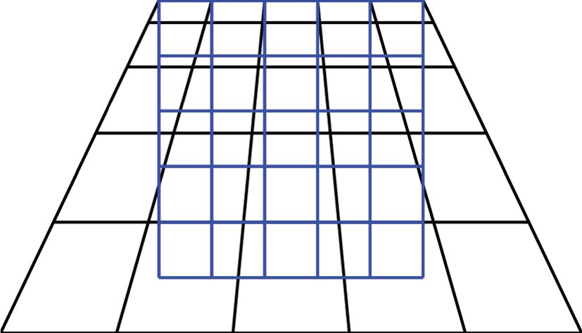
 A conceptual schematic of the trapezoid coordinate trans-
According to the theory of Wu et al. (2019b), the trapezoid formation is shown in figure 1. By using such transformation,
coordinate transformation is we can transform variable trapezoid grids in the Cartesian co-
 { x0 − ordinate system (figure 1 grid in black) to square grids in the
 x = 1+ (z) , trapezoid coordinate system (figure 1 grid in blue), and they
 (1)
 z0 = (z), cover the same subsurface region.
 595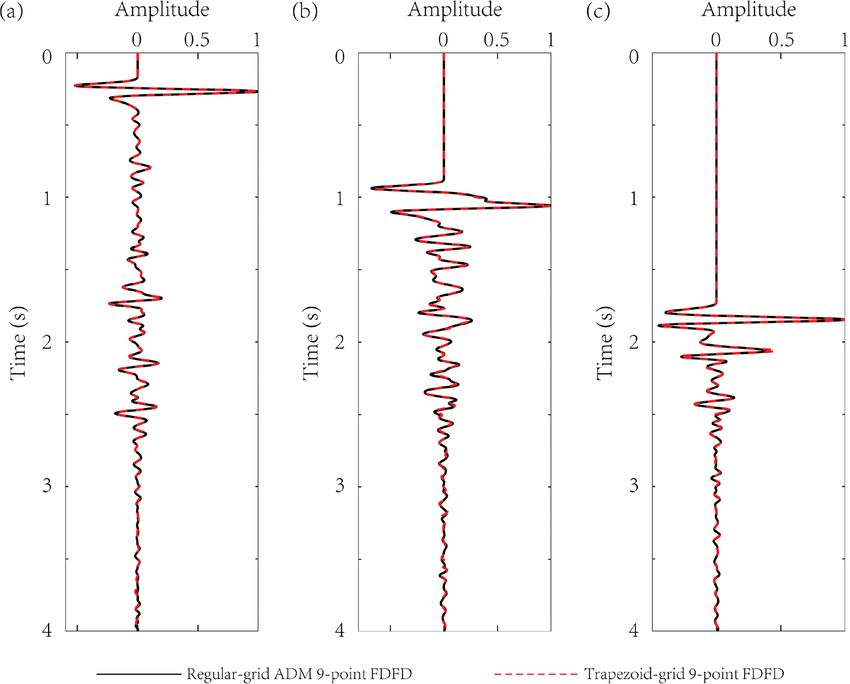

Journal of Geophysics and Engineering (2021) 18, 594–604 Wu et al.

 To reduce artificial boundary reflections, the PML
 (Berenger 1994) is adopted in modeling. The principle of
 PML is to add an absorbing medium around the simulating
 area and replace propagating waves with exponentially de-
 caying waves by analytically continuing the wave equation
 into complex coordinates (Gao et al. 2017) as follows:
 1 
 → , (7)
 x dx x

Figure 1. Meshes in the Cartesian coordinate system (black) and the where dx = 1 + (1∕i ) ln(1∕R)(3v
 √ max ∕2L)(̃ x∕L)2 is the
trapezoid coordinate system (blue). The two meshes cover the same phys- attenuation function, i = −1, L is the thickness of PML, R
ical subsurface region. is the theoretical reflection coefficients and x̃ is the distance
 from the inner area to the PML area. We can also apply the

 Downloaded from https://academic.oup.com/jge/article/18/4/594/6350127 by guest on 19 October 2021
2.2 Trapezoid coordinate system Helmholtz equation PML in the z-direction in the same way.
 Substituting equations (6) and (7) into equation (5),
The Cartesian coordinate system Helmholtz equation (Xu & we can obtain the trapezoid grid frequency-domain acoustic
Gao 2018) is equation with a PML absorbing boundary condition:
 2 2 2 
 − = + 2 + (x0 − x0s ) (z0 − z0s )f ( ),(4) 2 1 2 x2 + 1 2 1 2 2 x 
 v2 x20 z0 − = +
 v 2 dx [1 + (z)] x
 2 2 2 dx [1 + (z)] x
 2

where = ( , x0 , z0 ) is the wavefield function in the fre- ( 2 )
 1 x 2 
quency domain, (x0s , z0s ) is the position of the source term − −
in the Cartesian coordinate system and f( ) is the frequency- dx dz [1 + (z)] ′ (z) x′ 2 z′ 2
domain source function. ′′
 1 (z) 1 1 2 
 Using equation (1), we can derive the partial derivative − +
relation between the above two coordinate systems by the dz [ (z)]3 z d2z [ (z)]2 z2
 ′ ′

chain rule (Wu et al. 2019b). Then the trapezoid coordinate
 1 dx 2 x2 + 1 1 dz 1 
system Helmholtz equation can be given as − − 3
 dx x [1 + (z)] x dz z [ (z)] z
 3 2 ′ 2
 2 2 x2 + 1 2 2 2 x 
 − = + + (x − xs )(z − zs )f ( ).
 v 2 [1 + (z)] x
 2 2 [1 + (z)] x
 2 (8)
 ′′
 2 x 2 (z) 
 − − ′ 2.3 Trapezoid-grid 9-point FDFD scheme
 [1 + (z)] (z) x z [ (z)]3 z
 ′

 To balance the efficiency and the accuracy, the ADM (Chen
 1 2 2012) is used to approximate second-order spatial derivatives
 + ′ + (x − xs )(z − zs )f ( ),
 [ (z)]2 z2 2 / x2 , 2 / z2 and the mass acceleration term. For first-
 (5) order spatial derivatives / x, / z and second-order
 derivatives 2 ∕ x′2 , 2 ∕ z′2 , we use the second-order
where = ( , x, z) is the wavefield function and (xs , zs ) central difference for discretization.
is the position of the source term in the trapezoid coordinate As a result, we obtain the 9-point FDFD formula of equa-
system. tion (8) as follows:
 For the mixed partial derivative ( 2 )/( x z) in
equation (5), we use the 45◦ -rotated grid (Liu et al. 2
 − [c m,n + d( m−1,n + m+1,n + m,n−1 + m,n+1 )
2018; Wu et al. 2019b), which takes the transforma- v2m,n
tion x = x′ cos( ∕4) − z′ cos( ∕4), z = x′ sin( ∕4) +
z′ sin( ∕4), to transform it into non-mixed spatial deriva- + e( m+1,n+1 + m+1,n−1 + m−1,n+1 + m−1,n−1 )]
tives:
 ( ) 1 2 x2 + 1 ̄ m+1,n + ̄ m−1,n − 2 ̄ m,n
 2 1 2 2 =
 = − , (6) d2x [1 + (z)]2 Δx2
 x z 2 x′ 2 z′ 2
 2 2 x m+1,n − m−1,n
where x′ and z′ are coordinates in the diagonal directions of +
 1
the meshes (Liu et al. 2018; Wu et al. 2019b). dx [1 + (z)]2 2Δx
 596

Journal of Geophysics and Engineering (2021) 18, 594–604 Wu et al.
 1 x Substituting equation (12) into equation (9), we have
 −
 dx dz [1 + (z)] ′ (z) 2 x2 + 1
 [2a(T4 − 1) + (1 − a)T1 (T3 − 1)
 m+1,n+1 + m−1,n−1 − m+1,n−1 − m−1,n+1 [1 + (z)]2
 ×
 Δx2 + Δz2 2 2 x
 + (1 − a)T2 (T5 − 1)] + (−iT7 Δx)
 1 (z) m,n+1 − m,n−1
 ′′
 1 1 [1 + (z)]2
 − ′
 + 2 ′
 dz [ (z)]3 2Δz dz [ (z)]2 x
 − (−iT1 T6 + iT2 T8 )
 [1 + (z)] ′ (z)
 ̂ m,n+1 + ̂ m,n−1 − 2 ̂ m,n 1 dx 2 x2 + 1
 × − ′′
 (z) Δz
 Δz2 d3x x [1 + (z)]2 − (T − T2 ) + ′
 1
 {T
 [ ′ (z)]3 2 1 [ (z)]2 1
 m+1,n − m−1,n 1 dz 1 m,n+1 − m,n−1
 × − × [(1 − b)T3 + b] + T2 [(1 − b)T5 + b]
 dz z [ (z)]
 ′

 Downloaded from https://academic.oup.com/jge/article/18/4/594/6350127 by guest on 19 October 2021
 2Δx 3 2 2Δz
 − 2[(1 − b)T4 + b]}
 + (x − xs )(z − zs )f ( ), (9)
 4 2
where + [c + d(2T4 + T1 + T2 )
 G2x [1 + (z)]2
 1−a 1−a
 ̄ m,n =
 0
 m,n+1 + a m,n + m,n−1 ,
 2 2 + 2e(T1 T3 + T2 T5 )] = 0, (13)
 1−b 1−b
 ̂ m,n = m+1,n + b m,n + m−1,n , where
 2 2
 m, n = (mΔx, nΔz), vm, n = v(mΔx, nΔz) and Δx and {
 2 (z + Δz) − (z)
Δz are intervals in corresponding directions. The coefficients T1 = exp −i
 G∗x Δx 1 + (z)
c = 0.6348, d = 0.0913, e = (1 − c − 4d)/4 and a = b = 0.7944 0

are the same as those in Chen (2012). }
 [ x sin( ) + cos( )] ,
 {
2.4 Dispersion analysis 2 (z − Δz) − (z)
 T2 = exp −i
 G∗x Δx 1 + (z)
In this subsection, we conduct an analysis of the dispersion 0

relation of our trapezoid-grid FDFD method. }
 The theoretical plane wave solution of the 2D Helmholtz [ x sin( ) + cos( )] ,
equation (Xu & Gao 2018) can be described as { }
 2 1 + (z + Δz)
 T3 = cos sin( ) ,
 0 e−ik sin( )x0 −ik cos( )z0 , (10) G∗x
 0
 1 + (z)
where 0 is a constant, k = ∕v = (2 )∕(Gx0 Δx0 ) repre- { }
 2 
sents the theoretical wave number, is the propagation angle T4 = cos sin( ) ,
 G∗x
 { }
 0
of acoustic wave in the Cartesian coordinate system and Gx0
 2 1 + (z − Δz)
is the theoretical NPPW in the x0 -direction. T5 = cos sin( ) ,
 To give the dispersion relation of our method, we as- G∗x 1 + (z)
 { }
 0

sume the numerical plane wave solution corresponding to 2 1 + (z + Δz)
 T6 = sin sin( ) ,
our FDFD scheme has a form as G∗x 1 + (z)
 0

 ∗0 e−ik
 ∗ sin( )x0 −ik∗ cos( )z0
 , (11) { }
 2 
 T7 = sin sin( ) ,
where k∗ = ∕vph = (2 )∕(G∗x Δx0 ) represents the numer- G∗x
 { }
 0

 2 1 + (z − Δz)
 0
ical wave number, vph is the phase velocity and G∗x represents T8 = sin sin( ) .
 0
the given number of NPPW in the x0 -direction. G∗x 1 + (z)
 0
 According to the coordinate transformation in equa-
 We assume that for a given G∗x , Gx0 satisfies equation (13)
tion (1), we can get the numerical plane wave solution in the 0
 and is in the neighborhood of G∗x . Therefore, by minimizing
trapezoid coordinate system: 0
 the modules of equation (13), we can obtain Gx0 , and then
 ∗ sin( )[1+ (z)]x−ik∗ cos( ) (z)
 ∗0 e−ik , (12) get the normalized phase velocity vph ∕v = Gx0 ∕G∗x .
 0

 597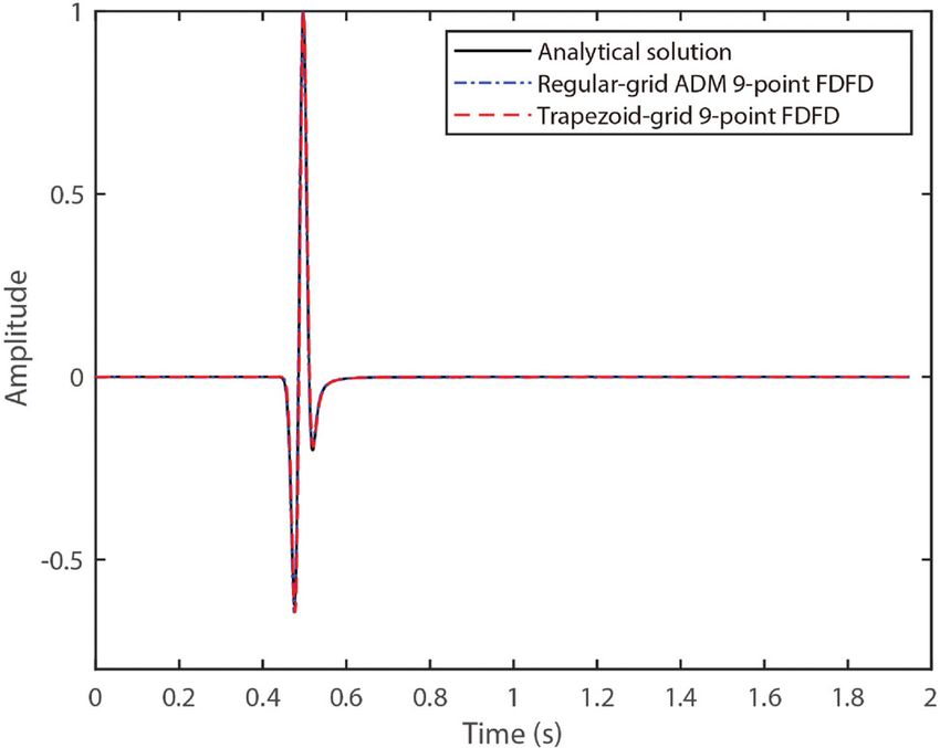

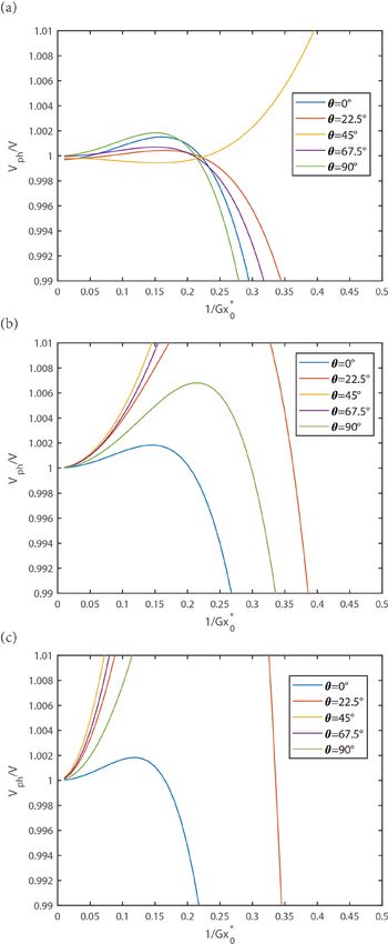
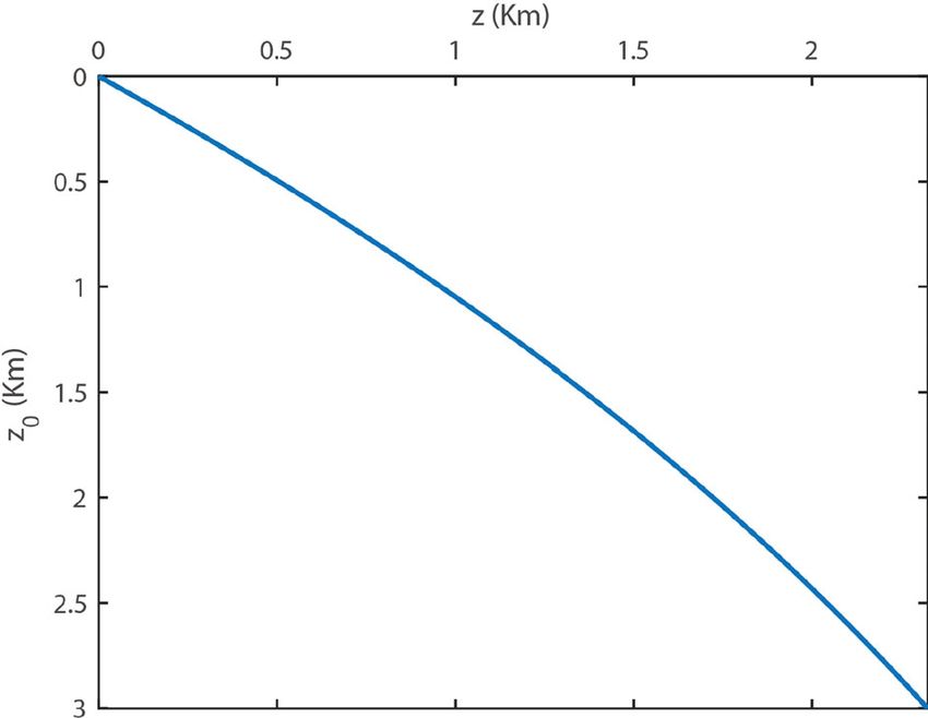
Journal of Geophysics and Engineering (2021) 18, 594–604 Wu et al.

 Downloaded from https://academic.oup.com/jge/article/18/4/594/6350127 by guest on 19 October 2021
Figure 2. The sampling function in depth for the Marmousi model.

 The dispersion of our method is not only related to the
NPPW, but also related to , (z), x and z. We choose the
trapezoid transformation parameters in the Marmousi model
as an example to show the corresponding dispersion curves.
The sampling function (z) is shown in figure 2 and is
1.4101 × 10−4 . To demonstrate the influences of x, z on
dispersion, we choose three spatial locations; (0 m, 0 m),
(1500 m, 1100 m) and (3000 m, 2200 m). The dispersion
curves are shown in figure 3, where the different lines in dif-
ferent colors represent the dispersion curves for different val-
ues of propagation angle in equation (12). Figure 3 in-
dicates that the required NPPW (for phase velocity error
less than 1%) increases with depth, which is the main lim-
itation of the proposed method. A possible way to further
improve the accuracy of the trapezoid-grid FDFD method
is to further optimise FDFD coefficients a, b, c, d and e in
equation (9).

3 Numerical test
Next, we will show the modeling results of our method for
three different models. The computational platform is an
Inter (R) Core (TM) i5-6300 HQ CPU, and MATLAB
codes are used. The modeling results of our trapezoid-
grid 9-point FDFD method are compared with the re-
sults of Chen’s regular-grid ADM 9-point FDFD method
(Chen 2012). The inverse Fourier transformation
 ∞ Figure 3. Dispersion curves of trapezoid-grid 9-point FDFD for the Mar-
 (t, x, z) = ∫−∞ ( , x, z)ei t d is used to transform mousi model at (x, z) = (a) (0 m, 0 m), (b) (1500 m, 1100 m) and (c)
the simulation results from the frequency domain to the (3000 m, 2200 m).
time domain.

3.1 Homogeneous model
 is 20 Hz. The spatial grid sizes in the Cartesian coordi-
The velocity of the homogeneous model is 3000 m s−1 , and nate system are Δx0 = Δz0 = 12.5 m, while the spatial
the size of this model is 2500 m × 2500 m. We set a Ricker sizes in the trapezoid coordinate system are Δx = Δz =
wavelet at (1250 m, 1250 m), and the dominant frequency 8.7719 m. We set = 1.7 × 10−4 and (z) = z at this model.

 598

Journal of Geophysics and Engineering (2021) 18, 594–604 Wu et al.

Figure 4. Monochromatic wavefields (real part) at 20 Hz for the homogeneous model: (a) regular-grid ADM 9-point FDFD; (b) trapezoid-grid 9-point

 Downloaded from https://academic.oup.com/jge/article/18/4/594/6350127 by guest on 19 October 2021
FDFD.

Figure 5. Wavefield snapshots at 0.52 s for the homogeneous model: (a) regular-grid ADM 9-point FDFD; (b) trapezoid-grid 9-point FDFD.

The PML absorbing boundary with a thickness of 300 m
is used.
 Figures 4a and b give the real part of the monochromatic
wavefields at 20 Hz calculated by the regular-grid ADM 9-
point FDFD and our method, respectively. Figure 4 shows
a good agreement between the two monochromatic wave-
fields. Figure 5 compares the snapshots of the regular-grid
ADM 9-point FDFD and trapezoid-grid 9-point FDFD at
0.52 s and there is no visible difference. Figure 6 shows the
comparison between the signals recorded by the receiver lo-
cated at (1250 m, 0 m) and the analytical solution. Obviously,
the result of our method fits the analytical solution well.

3.2 Three-layer model
Secondly, we test using a three-layer model. The model is Figure 6. Signals recorded by receiver located at (1250 m, 0 m) for the ho-
exhibited in figure 7a, and the region covered by red lines mogeneous model.
represents the actual simulating area for the trapezoid-grid
FDFD method. The sampling function in depth is shown The spatial grids sizes in the Cartesian coordinate system are
in figure 7b. We set a Ricker wavelet at (1250 m, 0 m), and Δx0 = Δz0 = 12.5 m, while the spatial sizes in the trapezoid
the dominant frequency is 20 Hz. We set 141 receivers at the coordinate system are Δx = Δz = 10.9608 m, and = 1.6923
surface of the model from (375 m, 0 m) to (2125 m, 0 m). × 10−4 .

 599

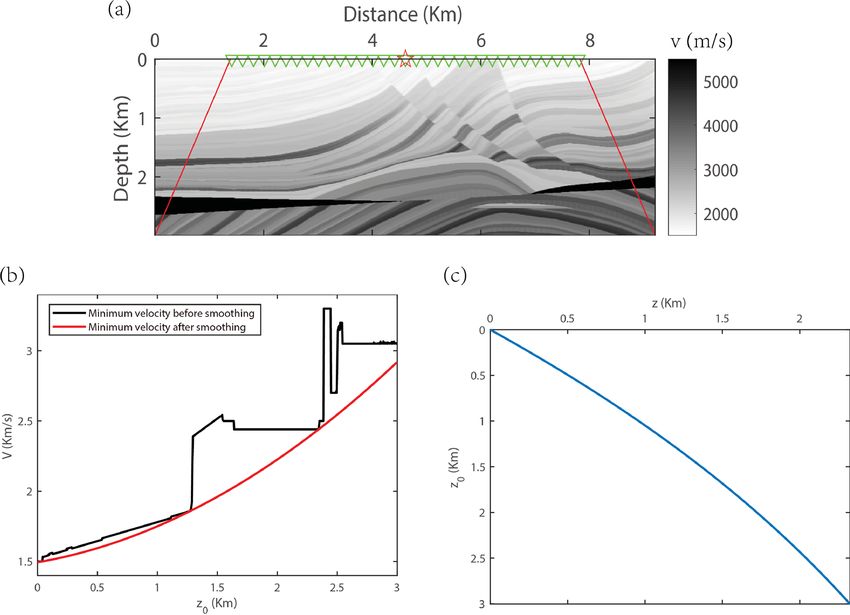
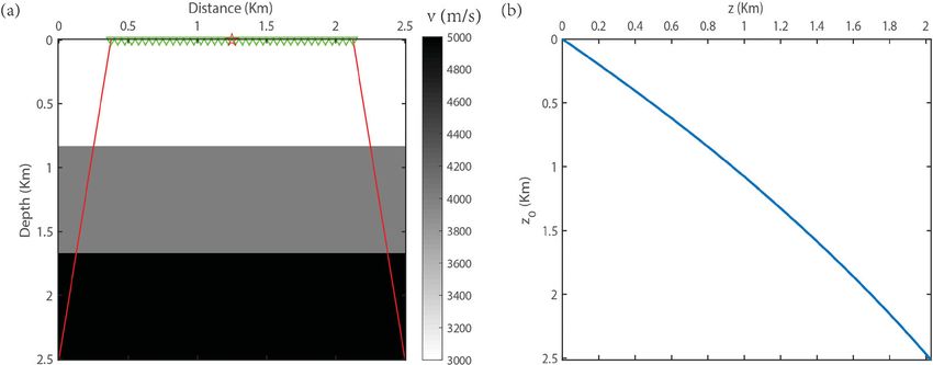
Journal of Geophysics and Engineering (2021) 18, 594–604 Wu et al.

Figure 7. (a) Three-layer model. The region covered by red lines represents the actual simulating area when using trapezoid-grid FDFD method. The

 Downloaded from https://academic.oup.com/jge/article/18/4/594/6350127 by guest on 19 October 2021
green triangles at the surface are receivers. The red star at the center of surface is the source. (b) Sampling function g(z) for the three-layer model.

Figure 8. Monochromatic wavefields (real part) at 20 Hz for the three-layer model: (a) regular-grid ADM 9-point FDFD; (b) trapezoid-grid 9-point
FDFD.

Figure 9. Recorded seismograms for the three-layer model: (a) regular-grid ADM 9-point FDFD; (b) trapezoid-grid 9-point FDFD.

 Figures 8a and b give the real part of the monochro- larity verifies the effectiveness of our method for the layered
matic wavefields at 20 Hz calculated by regular-grid ADM 9- model.
point FDFD and our method, respectively. Figures 9a and
b give the seismograms of the regular-grid ADM 9-point
FDFD and the trapezoid-grid 9-point FDFD, respectively. 3.3 Marmousi model
We can see the direct wave and the reflected wave clearly.
The comparison between wavefield snapshots at 0.62 s of Finally, we show the numerical results of our method for the
the above schemes are shown in figure 10, and their simi- Marmousi model (figure 11a). The region covered by red

 600

Journal of Geophysics and Engineering (2021) 18, 594–604 Wu et al.

 Downloaded from https://academic.oup.com/jge/article/18/4/594/6350127 by guest on 19 October 2021
Figure 10. Wavefield snapshots at 0.62 s for the three-layer model: (a) regular-grid ADM 9-point FDFD; (b) trapezoid-grid 9-point FDFD.

lines in figure 11a represents the actual simulating area for points and computational time of regular-grid ADM 9-point
the trapezoid-grid FDFD method. We set a Ricker wavelet at FDFD and trapezoid-grid 9-point FDFD are given in Table 1.
(4612.5 m, 0 m), and the dominant frequency is 10 Hz. We It shows that trapezoid-grid FDFD method can not only de-
set 517 receivers at the surface of the model from (1375 m, crease about 80% computational time but also save about
0 m) to (7825 m, 0 m). The spatial grids sizes in the Carte- 80% computer memory compared with a regular-grid ADM
sian coordinate system are Δx0 = 12.5 m and Δz0 = 4 m, FDFD method.
while the spatial sizes in the trapezoid coordinate system are Figures 12a and b give the real part of the monochro-
Δx = Δz = 12.4297 m, and = 1.4101 × 10−4 . The grid matic wavefields at 10 Hz calculated by the regular-grid

Figure 11. (a) Marmousi model. The region covered by red lines represents the actual simulating area when using trapezoid-grid FDFD method. The
green triangles at surface are receivers. The red star at the center of surface is the source. (b) The minimum velocity function vmin (g(z)) for the Marmousi
model; the black line represents the function before smoothing and the red line represents the function after smoothing. (c) Sampling function g(z) for
the Marmousi model.

 601

Journal of Geophysics and Engineering (2021) 18, 594–604 Wu et al.
Table 1. Grid points and computational time for the Marmousi model.

FDFD scheme Grid points Time

Regular-grid ADM 9-point FDFD 737 × 750 20.0063 s
Trapezoid-grid 9-point FDFD 521 × 188 3.4861 s

 Downloaded from https://academic.oup.com/jge/article/18/4/594/6350127 by guest on 19 October 2021
 Figure 14. Wavefield snapshots at 1 s for the Marmousi model: (a)
 regular-grid ADM 9-point FDFD; (b) trapezoid-grid 9-point FDFD.

 most the same accuracy as the regular-grid ADM 9-point
 FDFD.

Figure 12. Monochromatic wavefields (real part) at 10 Hz for the Mar-
mousi model: (a) regular-grid ADM 9-point FDFD; (b) trapezoid-grid 9- 4 Conclusion
point FDFD.
 In this paper, we have explored the trapezoid-grid FDFD
 seismic wave simulation method. We derive the trapezoid
ADM 9-point FDFD and our method, respectively. Figure 12 coordinate system Helmholtz equation and the correspond-
shows a good agreement between two monochromatic wave- ing PML absorbing boundary condition. To balance the
fields. Transforming the frequency domain results into the efficiency and the accuracy of the numerical scheme, we
time domain via Fourier transform, we get the seismo- combine the ADM and the central difference to discretise
grams of the regular-grid ADM (figure 13a) and our method the above equation. We also make a dispersion analysis for
(figure 13b). The comparison of snapshots at 1 s and 2 s our method, which indicates that our trapezoid-grid 9-point
for the above two methods are shown in figure 14 and fig- FDFD method can satisfy the requirement of the maximum
ure 15, respectively. To make a detailed comparison, we ex- phase velocity error being less than 1% with appropriate pa-
tract the trace at 4.4375 km (figure 16a), 5.9750 km (fig- rameters. Numerical tests on the homogeneous model and
ure 16b) and 7.500 km (figure 16c) from figure 13. Figure 16 the layered model verify the correctness and effectiveness
shows that our trapezoid-grid 9-point FDFD can achieve al- of our method. Numerical tests on the Marmousi model

Figure 13. Recorded seismograms for the Marmousi model: (a) regular-grid ADM 9-point FDFD; (b) trapezoid-grid 9-point FDFD.

 602

Journal of Geophysics and Engineering (2021) 18, 594–604 Wu et al.

 Acknowledgments
 This work was supported by Natural Science Basic Research
 Program of Shaanxi (grant no. 2020JM-018). The work of
 the third author was also sponsored by the China Scholarship
 Council (grant no. 201906280270) during his visit to Duke
 University.

 References
 Berenger, J.P., 1994. A perfectly matched layer for the absorption of elec-
 tromagnetic waves, Journal of Computational Physics, 114, 185–200.
 Chen, F. & Xu, S., 2012. Pyramid-shaped grid for elastic wave propaga-
 tion, Society of Exploration Geophysicists Technical Program Expanded
 Abstracts, 1–5.

 Downloaded from https://academic.oup.com/jge/article/18/4/594/6350127 by guest on 19 October 2021
 Chen, J., 2012. An average-derivative optimal scheme for frequency-
 domain scalar wave equation, Geophysics, 77, T201–T210.
Figure 15. Wavefield snapshots at 2 s for the Marmousi model: (a) Chung, W., Pyun, S., Bae, H.S. & Shin, C., 2011. Frequency-domain
regular-grid ADM 9-point FDFD; (b) trapezoid-grid 9-point FDFD. elastic reverse-time migration using wave-field separation, Society
 of Exploration Geophysicists Technical Program Expanded Abstracts,
show that, compared with the regular-grid ADM 9-point 3419–3424.
 da Costa, F.T., Santos, M.A.C. & Soares Filho, D.M. 2020. Wavenumbers
FDFD, our method can achieve a significant reduction in illuminated by time-domain acoustic FWI using the L1 and L2 norms,
both CPU time and computer memory while keeping a sim- Journal of Applied Geophysics, 174, 103935.
ilar level of accuracy. Therefore, our trapezoid-grid FDFD Dablain, M.A., 1986. The application of high-order differencing to the
method can further improve the efficiency of seismic wave scalar wave equation, Geophysics, 51, 54–66.
simulations. Fan, N., Zhao, L., Xie, X., Tang, X. & Yao, Z., 2017. A general optimal
 method for a 2D frequency-domain finite-difference solution of scalar
 The key idea of our method is the combination of the
 wave equation, Geophysics, 82, T121–T132.
trapezoid grid with FDFD stencils. Such an idea can be gener- Fan, N., Zhao, L., Xie, X. & Yao, Z., 2018. A discontinuous-grid finite-
alised to many other wave equations such as the 3D acoustic difference scheme for frequency-domain 2D scalar wave modeling,
equation and the 3D elastic equation. Geophysics, 83, T235–T244.

Figure 16. Single trace comparisons for figure 13 at three different locations: (a) 4.475 km; (b) 5.9750 km; (c) 7.500 km.

 603

Journal of Geophysics and Engineering (2021) 18, 594–604 Wu et al.

Gao, J., Xu, W., Wu, B., Li, B. & Zhao, H., 2018. Trapezoid grid finite differ- finite difference (RBF-FD) algorithm with hybrid kernels, Society of
 ence seismic wavefield simulation with uniform depth sampling interval, Exploration Geophysicists Technical Program Expanded Abstracts, 4022–
 Chinese Journal of Geophysics, 61, 3285–3296. 4027.
Gao, Y., Song, H., Zhang, J. & Yao, Z., 2017. Comparison of artificial ab- Shi, Y., Zhang, W. & Wang, Y., 2019. Seismic elastic RTM with vector-
 sorbing boundaries for acoustic wave equation modelling, Exploration wavefield decomposition, Journal of Geophysics and Engineering, 16,
 Geophysics, 48, 76–93. 509–524.
Herman, A.J., Anania, R.M., Chun, J.H., Jacewitz, C.A. & Pepper, R.E.F., Takekawa, J. & Mikada, H., 2018. A mesh-free finite-difference method for
 1982. A fast three-dimensional modeling technique and fundamen- elastic wave propagation in the frequency-domain, Computers and Geo-
 tals of three-dimensional frequency-domain migration, Geophysics, 47, sciences, 118, 65–78.
 1627–1644. Tan, W., Wu, B., Li, B. & Lei, J., 2020. Seismic wave simulation using a
Hu, J. & Jia, X., 2016. Numerical modeling of seismic waves using trapezoid grid pseudo-spectral method, Oil Geophysical Prospecting, 55,
 frequency-adaptive meshes, Journal of Applied Geophysics, 131, 41–53. 1282–1291 (in Chinese).
Hu, Y., Han, L., Wu, R. & Xu, Y., 2019. Multi-scale time-frequency domain Wang, E., Ba, J. & Liu, Y., 2018. Time-space-domain implicit finite-
 full waveform inversion with a weighted local correlation-phase misfit difference methods for modeling acoustic wave equations, Geophysics,
 function, Journal of Geophysics and Engineering, 16, 1017–1031. 83, T175–T193.
Huang, C. & Dong, L., 2009a. High-order finite-difference method in seis- Wang, E., Ba, J. & Liu, Y., 2019. Temporal high-order time-space domain

 Downloaded from https://academic.oup.com/jge/article/18/4/594/6350127 by guest on 19 October 2021
 mic wave simulation with variable grids and local time-steps, Chinese finite-difference methods for modeling 3d acoustic wave equations on
 Journal of Geophysics, 52, 176–186. general cuboid grids, Pure and Applied Geophysics, 176(12).
Huang, C. & Dong, L., 2009b. Staggered-grid high-order finite-difference Wu, B., Xu, W., Jia, J., Li, B., Yang, H., Zhao, H. & Gao, J., 2018. Con-
 method in elastic wave simulation with variable grids and local time- volutional perfect-matched layer boundary for trapezoid grid finite-
 steps, Chinese Journal of Geophysics, 52, 1324–1333. difference seismic modeling, Society of Exploration Geophysicists Techni-
Jia, J., Zhao, Q., Xu, Z., Meng, D. & Leung, Y., 2021. Variational Bayes’ cal Program Expanded Abstracts, 3989–3993.
 method for functions with applications to some inverse problems, SIAM Wu, B., Li, B., Yang, H. & Jia, J., 2019a. Trapezoid grid finite difference
 Journal on Scientific Computing, 43, A355–A383. for acoustic wave modeling, in Society of Exploration Geophysicists Seis-
Jo, C.H., Shin, C. & Suh, J.H., 1996. An optimal 9-point, finite-difference, mic Imaging Workshop, Beijing, China, 2018, Society of Exploration
 frequency-space, 2-D scalar wave extrapolator, Geophysics, 61, 529–537. Geophysicists, p. 52.
Liu, X., Greenhalgh, S., Zhou, B. & Greenhalgh, M., 2018. Frequency- Wu, B., Xu, W., Li, B. & Jia, J., 2019b. Trapezoid coordinate finite difference
 domain seismic wave modelling in heterogeneous porous media us- modeling of acoustic wave propagation using the CPML boundary con-
 ing the mixed-grid finite-difference method, Geophysical Journal Inter- dition, Journal of Applied Geophysics, 168, 101–106.
 national, 216, 34–54. Xu, W. & Gao, J., 2018. Adaptive 9-point frequency-domain finite differ-
Liu, Y., Liu, W., Yang, J. & Dong, L., 2021. Extracting angle domain com- ence scheme for wavefield modeling of 2D acoustic wave equation, Jour-
 mon image gather with variable density acoustic-wave equation, Journal nal of Geophysics and Engineering, 15, 1432–1445.
 of Geophysics and Engineering, 18, 192–199. Yang, H., Jia, J., Wu, B. & Gao, J., 2018. Mini-batch optimized full wave-
Luo, J., Wu, R., Hu, Y. & Chen, G., 2021. Strong scattering elastic full form inversion with geological constrained gradient filtering, Journal of
 waveform inversion with the envelope Fréchet derivative, Institute of Applied Geophysics, 152, 9–16.
 Electrical and Electronics Engineers Geoscience and Remote Sensing Letters, Zhang, Y., Gao, J. & Peng, J., 2018. Variable-order finite difference scheme
 doi:10.1109/LGRS.2021.3061972. for numerical simulation in 3-D poroelastic media, Institute of Electrical
Mishra, P., Nath, S., Fasshauer, G. & Sen, M., 2017. Frequency-domain and Electronics Engineers Transactions on Geoscience and Remote Sensing,
 meshless solver for acoustic wave equation using a stable radial basis- 56, 2991–3001.

 604