Short-term forecasts of COVID-19 spread across Indian states until 1 May 2020 - arXiv

Short-term forecasts of COVID-19 spread across Indian states

 until 1 May 2020
Neeraj Poonia1, Sarita Azad2*

1
 School of Basic Sciences, Indian Institute of Technology Mandi, 175075, India.
2
 School of Basic Sciences, Indian Institute of Technology Mandi, 175075, India.

*Corresponding author sarita@iitmandi.ac.in

Abstract

The very first case of corona-virus illness was recorded on 30 January 2020, in India and the number
of infected cases, including the death toll, continues to rise. In this paper,
we present short-term forecasts of COVID-19 for 28 Indian states and five union territories using real-
time data from 30 January to 21 April 2020. Applying Holt’s second-order exponential smoothing
method and autoregressive integrated moving average (ARIMA) model, we generate 10-day ahead
forecasts of the likely number of infected cases and deaths in India for 22 April to 1 May 2020. Our
results show that the number of cumulative cases in India will rise to 36335.63 [PI 95% (30884.56,
42918.87)], concurrently the number of deaths may increase to 1099.38 [PI 95% (959.77, 1553.76)]
by 1 May 2020. Further, we have divided the country into severity zones based on the cumulative
cases. According to this analysis, Maharashtra is likely to be the most affected states with around
9787.24 [PI 95% (6949.81, 13757.06)] cumulative cases by 1 May 2020. However, Kerala and
Karnataka are likely to shift from the red zone (i.e. highly affected) to the lesser affected region. On
the other hand, Gujarat and Madhya Pradesh will move to the red zone. These results mark the states
where lockdown by 3 May 2020, can be loosened.

Keywords: COVID-19; India; Prediction models; Statistics; Data; Indian states.

1 Introduction
COVID-19 illness, an on-going epidemic, started in Wuhan city, China, in December 2019
continues to cause infections in many countries around the world [1]. Considering the scale
and speed of transmission of COVID-19, on 11 March 2020, the World Health Organization
(WHO) declared it as a pandemic [2]. Thereafter, COVID-19 has become a threat to human
life on the planet. It has shown rapid infections in almost all countries, and there is no cure
available for this deadly virus. Presently governments have issued precautionary measures
such as social distancing, sanitization of streets and markets, quarantine of suspected and
infected cases, and lockdown of the communities at different scales (colonies, towns, states,
and countries, etc.). In India, exponential growth has not been observed as compared to the
USA and other European countries. It is due to the measures taken by the Indian government.
It indicates that there is a strong influence of these measures, such as lockdown on the
transmission behavior of COVID-19. On the other side, these measures create substantial
economic losses to the communities, and hence actions mentioned above cannot be imposed
for longer periods. Mainly, developing countries (such as India) cannot afford such payoff
after some finite time. The Indian government has continuously reviewed every hour
situation in every state. The government has become more focused on localizing the
lockdown in particularly alarming states and few towns which are hotspots for COVID-19.
For all these, it is important to have short-term forecasts which can be steering point for
decision-makers and administrations. In this connection, data-based statistical models such as
Autoregressive integrated moving average (ARIMA) and Holts method have shown

 1

effectiveness in predicting short-term forecast including the dengue fever [3, 4], the
hemorrhagic fever with renal syndrome [5], Tuberculosis [6] and COVID-19 [7]. ARIMA
has more ability compared to other prediction models like the support vector machine and
wavelet neural network for drought forecasting [8]. Also, exponential smoothing methods
have been widely used for forecasting of the population in West Java [9], an inflation rate of
Zambia [10] including a prediction for epidemic mumps [11] and COVID-19 [12–17].
However, mainly, for India, the short-term forecast is not done thoroughly. As India has
diversity across the states, it will be essential to study the spreading behavior of COVID-19
in different Indian states. This article presents a short-term forecast for various Indian states
which are severely infected.
 The main objective of the present paper is to present 10-day ahead forecasts from
22April to 1 May 2020 of the cumulative number of infected cases and deaths due to
COVID-19. This work also presents the analysis of Indian states at the regional level to
understand the spread of infection. The current situation of India is shown in Figure 1, with
the cumulative number of infected cases and deaths from 30 January to 21April 2020.

 Figure 1: (a) Number of infected cases from 30 Januaryto 21 April 2020; (b) Number of
 deaths from 30 January to 21 April 2020.

2 Materials and Methods

2.1ARIMAModel

The process whose statistical properties do not change with time, i.e. process with constant mean and
constant variance, known as a stationary process, is a crucial collection of stochastic processes.
Mathematically, the joint distribution of X (t1 ),..., X (t k ) and X (t1 ),..., X (t k  ) is the same for all
t1 , t 2 ,..., t k of a stationary process. Simply put, shifting the origin of time by a quantity  does not
change the statistical properties of the process. Usually, dealing with real-time data, most time series
does not exhibit stationarity in nature as they have no fixed mean. The properties of the crucial
collection of models for which the d th difference of the time series is a stationary mixed
autoregressive moving average process (ARMA). These models are known as ARlMA models. The
ARMA model, introduced by Box and Jenkins, is the collection of popular methods that are directly
applicable to modeling and analyzing the time series [18]. The ARMA model is formed by the merger
of two models, the autoregressive AR(p) model and the moving average MA(q) model. These models
are directly applicable to time series with stationary behavior. In case the series is non-stationary, it
must be dealt via differencing to make it stationary. Generally, the ARMA model after differencing is
known as ARIMA (p, d,q). Addressing

 H t   d X t  (1  k ) d X t (1)

 2

The general ARIMA model is given by

 H t  1 H t 1  ...   p H t  p  J t  ...   q J t q (2)

Hence, the ARIMA model can be written as

 f (k ) H t  g (k ) J t (3)
 f (k ) X t  g (k ) J t
 d
 (4)
The expressions in the Eq. 4 are defined as: f (k ), g (k ) are polynomials of degree p, qrespectively s.t.
 f (k )  1  1k  ...   p k p (5)
and
 g (k )  1  1k  ...   q k q (6)

While,  d is an operator, known as difference operator, and used to make the difference of time
series stationary; and d is the difference value. In real-time data, taking the first difference (d=1) is
usually found to be sufficient and occasionally second difference (d=2) would be enough to achieve
stationarity.
Akaike Information Criterion (AIC) is one of the essential criteria to select betweencompeting
models. Mathematically,
  T 
   et 
 AIC = log  t 1   2p (7)
  T  T
  
  
The model which has the least AIC is selected as the best model. Autocorrelation functions (ACF)
and partial autocorrelation functions (PACF) are used to select order of moving average process
MA(q) and autoregressive process AR(p) respectively. In the process to investigate the stationarity of
time series Kwiatkowski–Phillips–Schmidt–Shin (KPSS) [19] and Augmented Dickey-Fuller (ADF)
[20] tests are used. To reject the null hypothesis, the p-value must be smaller than the significance
level.

2.2 Holt’sMethod
The numbers of confirmed cases and deaths in India are increasing day by day, as shown in Figure 1
thereupon the time series exhibit trend. Simple exponential smoothing methods should not apply in
this case. When data shows the pattern, and there is no seasonality, Holt's method is a primary tool to
handle it. Holt's method is a double exponential smoothing method (not based on ARIMA approach)
which has two parameters. This method divides the time series into two sections: the level and the
trend denoted by Bt and M t respectively. These two parts are as follows:
 Bt  X t  (1   )( Bt 1  M t 1 ) (8)
 M t   ( Bt  Bt 1 )  (1   )M t 1 (9)
The in-future forecasts values X t h of the time series can be calculated by:
 X t h  Bt  M t (h) (10)

where h is the number of periods in the future. Diverse statistical meaning-making models in the R-
language platform were used to evaluate the time series of infected cases and deaths for prediction
purposes.

3. Results and Discussion

 3

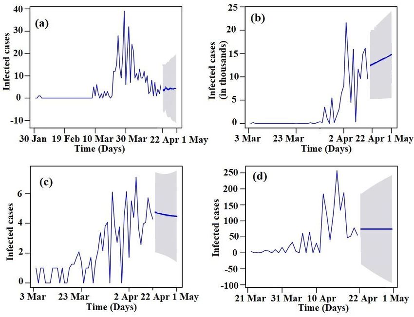
We present results for 10-day ahead forecasts (22 April to 1 May2020) generated for the
cumulative number of infected cases and deaths in India as well as in the ten most affected
states: Kerala, Maharashtra, Delhi, Gujarat, Tamil Nadu, Telangana, Uttar Pradesh, Madhya
Pradesh, Karnataka, Rajasthan. In this work, we used two models Holt's method and ARIMA
model to forecast the cumulative infected cases and deaths of COVID-19. For the ARIMA
model, we forecast per day new infected case(s) and new death(s), whereas for Holt’s method
cumulative numbers are generated.

3.1 Validation: As of12 April 2020, there were 9205 cumulative numbers of infected cases
and 331 cumulative numbers of deaths in India. For validation purposes, we forecasted the
cumulative number of infected cases and deaths from 7-12 April 2020, using ARIMA and
Holt's method. Our forecasting results showed 8064 [PI 95% (6743, 9842)] cumulative
number of infected cases using ARIMA(1,1,0) model and 8936 [PI 95% (7424, 10588)] cases
using Holt's method (α=0.9464, β=0.4311), in both cases the 95% prediction intervals
includes the actual values. While forecasting results of the cumulative number of deaths are
287 [PI 95% (210, 377)] using Holt's method (α=0.8052, β=0.2905) which includes the actual
value within 95% prediction interval but ARIMA(0,1,1) underfit the data with 276 [PI 95%
(225, 326)] cumulative number of deaths. To stabilize the variance in Holt's and
ARIMA(1,1,0) square root transformation is used.

3.2 India forecasting:
3.2.1 ARIMA model: During the analysis and forecasting of a time series, it is good to plot
the time series data and pay attention to the unique features exhibited by the time series. It
gives direction to the researcher for choosing an appropriate modeling approach that directly
captures identified features. Before starting the procedure, there is a need to make the time
series stationary. To stabilize the variance, we used square root transformation on the infected
number of cases per day time series. For investigating the stationarity of time series, we take
the support of the KPSS and ADF test, and results are shown in Table 1. The first difference
of series, i.e. d=1, is optimum to make series reasonably stationary. Based on a 5%
significance level both the tests, ADF and KPSS, reject the hypothesis of stationarity of time
series without making any difference. Afterwards taking the first difference, both the criteria
agree on the stationarity of time series. Further, to estimate another two parameters of the
candidate model, the ACF and PACF of series, first difference, and square root
transformation are used. From Figure 2(a) and 2(b), the ACF display one spike, and the
PACF also displays one spike. Initially, on the bases of the number of spikes, we selected
ARIMA(1, 1, 1). Alternate models are also used to compete with the ARIMA(1,1,1) model.
All alternative models and their AIC values with the Ljung-Box test p-values are shown in
Table 2. A model with a minimal amount of AIC is to have well-behaved residuals. Finally,
we select ARIMA(1,1,2) for forecasting. In terms of the residuals, the ARIMA(1,1,2) model
passed the Ljung-Box test with p-values larger than 0.05 level of significance. Since
ARIMA(1,1,2) has the lowest AIC value, which means the residuals of ARIMA(1,1,2) are
much well behaved compared to other considered models. We examine that all the residuals
are scattered around zero mean with constant variance. Using this, ARIMA(1,1,2) model
observe 36335.53 [95% PI(30884.56 -42918.87)] cumulative infected cases between by 1
May2020, results are shown in Table 3.

 Table 1: Table of p-values from ADF and KPSS tests after taking the differences of square
 root transformed data for infected cases per day in India.

 Number of Difference ADF test (p-value) KPSS test (p-value)
 d=0 0.961 0.01

 4

d=1 0.01 0.058

Table 2: Potential models for infected cases per day with AIC value and Ljung-Box test p-
value.

 Model AIC value Ljung-Box test (p-value)
 ARIMA (0,1,2) 427.77 0.263
 ARIMA (1,1,2) 418.82 0.518
 ARIMA (0,1,1) 428.05 0.341
 ARIMA (1,1,1) 428.59 0.258
 ARIMA (1,1,3) 420.72 0.438

 Figure 2: (a) ACF for the infected number of cases per day after square root
 transformation; (b) PACF for the infected number of cases per day after square root
 transformation; (c) ACF for the number of deaths per day; (d) PACF for the number
 of deaths per day.

Table 3: Results of 10-days ahead forecasts (22 April to 1 May 2020) using ARIMA model
for the cumulative number of infected cases and deaths.

 Date Forecast of 95% PI for infected Forecast of 95% PI for deaths
 cumulative cases deaths per day
 cases
 22 April 2020 21507.35 (21099.49, 21983.68) 680.46 (671.04, 1004.66)
 23 April 2020 22980.52 (22145.61, 23956.81) 727.64 (708.79, 1061.28)
 24 April 2020 24498.87 (23213.42, 26004.80) 772.26 (741.49, 1117.82)
 25 April 2020 26061.76 (24297.82, 28133.38) 817.41 (773.69, 1175.92)
 26 April 2020 27668.50 (25393.68, 30348.45) 863.09 (805.46, 1235.49)
 27 April 2020 29318.42 (26496.10, 32655.88) 909.29 (836.87, 1296.49)
 28 April 2020 31010.80 (27600.44, 35061.35) 956.02 (867.97, 1358.85)

 5

29 April 2020 32744.95 (28702.47, 37570.28) 1003.28 (898.79, 1422.54)
 30 April 2020 34520.13 (29798.33, 40187.84) 1051.06 (929.39, 1487.52)
 1 May 2020 36335.63 (30884.56, 42918.87) 1099.38 (959.77, 1553.76)

Since only one difference makes the time series stationary, we conclude to take d=1. Results
of ADF and KPSS tests are presented in Table 4. From Figure 2(c) and 2(d), ACF
demonstrates two significant spikes, and PACF demonstrates zero significant spike. Based on
the number of spikes, we selected ARIMA (0, 1, 2). Alternate models were also used to
compete with the ARIMA (0,1,2) model. Details of other potential models along with AIC
values and Ljung-Box test p-values given in Table 5. Furthermore, to forecast the number of
deaths per day in India, we found ARIMA (0,1,3) a reasonable model among other
competitor models it has minimum AIC value. Furthermore, we found residuals are randomly
scattered around zero mean with non-changing variance with time. Also, ARIMA(0,1,3) does
not show a lack of fit with the Ljung-box test p-value larger than 0.05. Graphical results of
forecasting from infected cases and deaths are shown in Figure 3. Applying ARIMA(0,1,23),
1099.38 [95% PI(959.77-1553.76)] cumulative deaths are expected in coming 10 days in
India. Results for 10-day ahead forecast for per day infected cases, and deaths are shown in
Table 3. To eliminate the effect of square root transformation in per day infected cases we
take a square of forecasted observations.

 Table 4: Table of p-values from ADF and KPSS tests for deaths per day in India.

 Number of Difference ADF test (p-value) KPSS test (p-value)
 d=0 0.979 0.01
 d=1 0.01 0.058

 Table 5: Potential models for deaths per day data with AIC values and Ljung-Box test p-
 values.

 Model AIC value Ljung-Box test (p-
 value)
 ARIMA (0,1,3) 497.32 0.408
 ARIMA (1,1,4) 499.79 0.208
 ARIMA (0,1,2) 498.10 0.248
 ARIMA (1,1,2) 498.77 0.274
 ARIMA (1,1,3) 498.41 0.365

 6

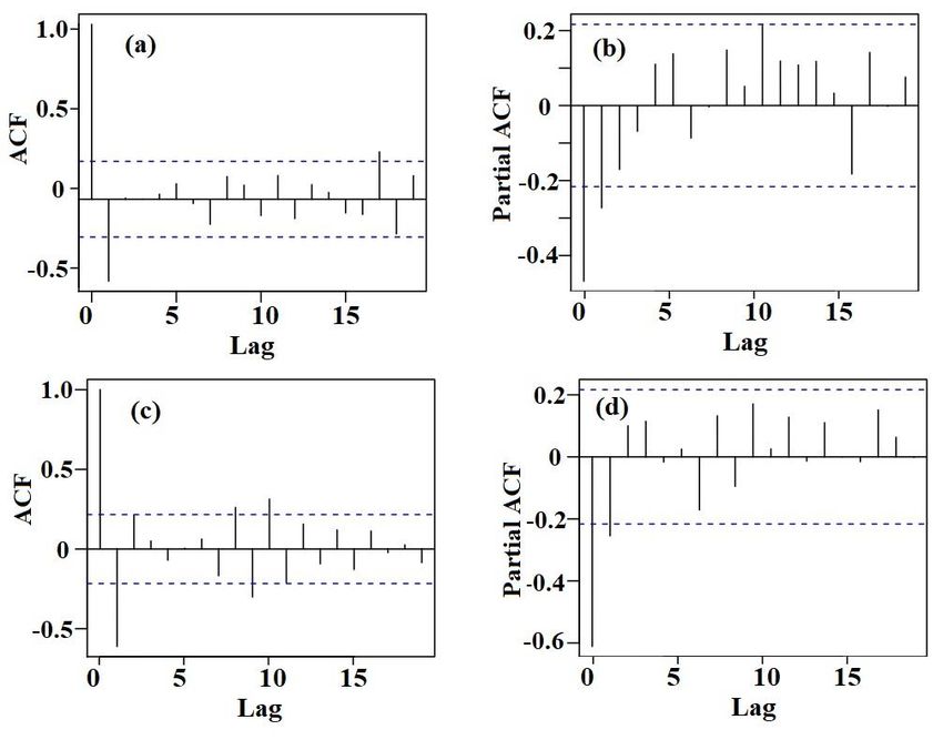
Figure 3: (a)10-days ahead forecast (22 April to 1 May 2020) for the number of
 infected cases per day using ARIMA(1,1,2) model; (b) 10-days ahead forecast (22
 April to 1 May 2020) for the number of deaths per day using ARIMA(0,1,3) model;
 (c) 10-days ahead forecast (22 April to 1 May 2020) using Holt's method for the
 cumulative number of infected cases; (d) 10-days ahead forecast (22 April to 1 May
 2020) for the cumulative number of days using Holt's method.

3.2.2 Holt's Method: The time series plot of the cumulative number of confirmed cases and
deaths for India is presented in Figure 1 exhibiting the trend in time series, but it does not
have a pattern of seasonality. As a result of the features shown by time series in Figure 1,
Holt’s method was selected in this study to accomplish a 10-day ahead forecast (22 April to 1
May 2020). Generally, a Holt method has two smoothing constants, α, and β (their values lie
in range 0 and 1). The square root transformation is used to stabilize the variance in the time
series of infected cases. In the process to attain the optimal parameters we applied by trial and
error technique. Results are shown in Table 6 with the value of α, β, AIC, and RMSE values.
The best model is selected with the lowest AIC and RMSE values. With the parameters,
α=0.9 and β=0.3, obtained values of AIC and RMSE are 381.02 and 1.05, respectively. For
this model, Ljung-Box test p-value=0.468 which agrees that model does not exhibit any lack
of fit.
 Using Holt's method, different values of α and β are tried to retrieve the optimum
forecast for cumulative deaths. The square root transformation is used to stabilize the
variance in the time series of deaths. The results of the trials are listed in Table 7 with AIC
and RMSE values. Smallest values of AIC=151.78 and RMSE=0.26 at α=0.8 and β=0.2 are
achieved. Subsequently, checking the Ljung-Box test p-value=0.109 we identify that model
does not lack of fit. Graphical results of forecasting from infected cases and deaths are
presented in Figure 3. From Table 8, 36624.43 [95% PI(30716.59-43051.56)] cumulative
infected cases and 1140.70 [ PI % (945.32-1354.42)] cumulative deaths are in India up-to 1
May2020.

 7

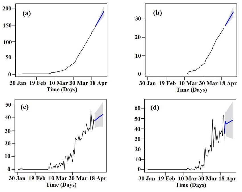
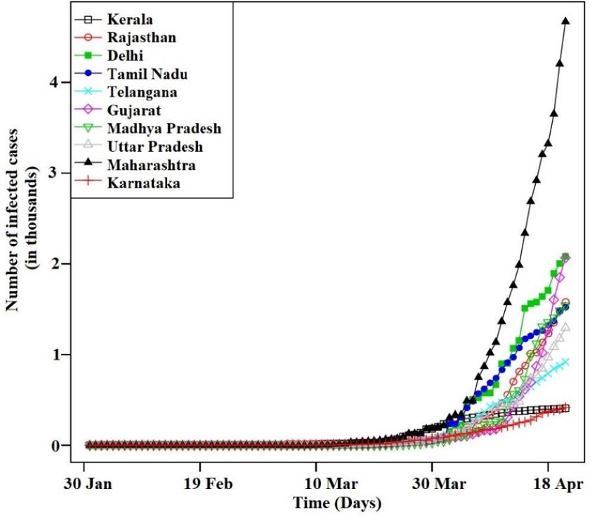
Table 6: Selection process for parameters in Holt’s method to forecast the cumulative
 number of infected cases in India.
 AIC value RMSE
 0.1 0.1 503.15 2.19
 0.5 0.1 435.19 1.46
 0.5 0.5 400.55 1.18
 0.9 0.5 383.37 1.06
 0.9 0.3 381.02 1.05

 Table 7: Selection process for parameters in Holt’s method to forecast the cumulative
 number of deaths.

 AIC value RMSE
 0.1 0.1 253.11 0.49
 0.5 0.1 185.53 0.32
 0.5 0.5 167.63 0.29
 0.9 0.5 157.12 0.27
 0.8 0.2 151.78 0.26

 Table 8: Results of 10-days ahead forecasts (22 April to 1 May 2020) using Holt’s method
 for the cumulative number of infected cases and deaths.

 Date Forecast of 95% PI for infected Forecast of 95% PI for deaths
 cumulative cases cumulative
 infected deaths
 cases
 22 April 2020 21498.39 (20883.67, 22122.02) 685.95 (658.43, 714.02)
 23 April 2020 22981.26 (21992.15, 23992.12) 730.79 (690.78, 771.94)
 24 April 2020 24513.58 (23102.62, 25966.35) 777.06 (723.16, 832.91)
 25 April 2020 26095.35 (24209.69, 28051.72) 824.75 (755.44, 897.10)
 26 April 2020 27726.57 (25311.47, 30251.70) 873.86 (787.58, 964.62)
 27 April 2020 29407.24 (26407.03, 32568.84) 924.39 (819.55, 1035.54)
 28 April 2020 31137.36 (27495.78, 35005.34) 976.34 (851.32, 1102.92)
 29 April 2020 32916.93 (28577.24, 37563.27) 1029.71 (882.88, 1187.82)
 30 April 2020 34745.95 (29650.98, 40244.67) 1084.49 (914.22, 1269.30)
 1 May 2020 36624.43 (30716.59, 43051.56) 1140.70 (945.32, 1354.42)

3.3 Indian states forecasting:
COVID-19 is spreading very fast in India. Locating the regions of most spread within India
will give insight for the lifting the lockdown which commenced on 25 March 2020. On the
regional level, this study shows the analysis for the cumulative number of cases but not
deaths due to the unavailability of data. A glimpse of the current situation of the increasing
number of cases in 10 states is given in Figure 4, certainly detectable that Maharashtra,
Gujarat, and Delhi are the most affected states in India till 21April2020. And Kerala is least
affected in our list of states. Time series starts from the date when the first case was reported
in the respective state.

 8

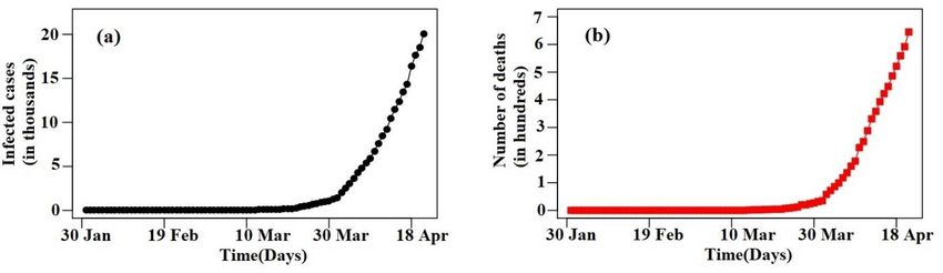
Figure 4: Number of infections in the ten most affected Indian states by corona-virus as of 30
 January to 21April2020.

3.3.1 ARIMA model: For forecasting purposes, using the ARIMA model, the number of
newly infected cases per day are analyzed instead of cumulative infected cases. To select the
optimum ARIMA model for each state, firstly each state's time series is made stationary by
taking differences. Next, we used ADF and KPSS tests to check stationarity. To stabilize the
variance of Delhi, Telangana, Uttar Pradesh, and Gujarat time series, cube root
transformations are used; later, one difference is enough to remove the trend. While to
stabilize the variance of Maharashtra, Karnataka and Rajasthan time series, square root and
square transformations are used, respectively.The same procedure is adopted for all the ten-
time series of infected cases per day. AIC values are used to select the best models, and the
model is chosen on the base of the smallest AIC value. Results of analysis for ARIMA
models are shown in Table 9. Analysis by ARIMA models shows that Maharashtra and
Gujarat will be the most affected states by 1 May2020, with around 9787.24 and
4216cumulative cases, respectively. As we observe that Kerala's growth is declining and it
will be less affected states with 449 [PI 95%(408-574.99)] cumulative cases. All the models
passed the Ljung-Box test as well as does not show any lack of fit.

 Table 9: Region-wise details of ARIMA models which were used for 10-days ahead forecasts
 (22 April to 1 May 2020), along with AIC values and Ljung-Box test p-values. Point forecasts
 and 95% prediction intervals are given in the last two columns.

 Region ARIMA AIC Ljung-Box Point 95% PI for infected
 Model value test forecast for cases
 (p-value) infected
 cases
 Kerala (2,1,0) 498.53 0.329 449.38 (408, 574.90)

 9

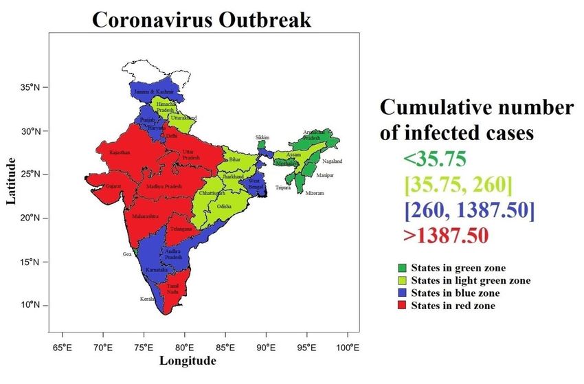
Maharashtra (0,1,2) 233.65 0.807 9787.24 (6949.81, 13757.06)
 Rajasthan (0,1,1) 947.38 0.147 2741.40 (2305.22, 3053.91)
 Delhi (1,1,2) 177.46 0.064 3039.73 (2139.72, 6085.18)
 Telangana (2,1,0) 133.99 0.112 1321.37 (940.84, 2740.89)
 Karnataka (3,1,0) 160.03 0.371 565.74 (419.09, 945.45)
 Gujarat (0,1,0) 89.76 0.131 4216.00 (2216.24, 13118.90)
 Uttar Pradesh (2,1,1) 140.25 0.161 2652.21 (1612. 43,4891.99)
 Tamil Nadu (1,1,1) 440.69 0.840 2157.35 (1520, 2878.82)
 Madhya Pradesh (0,1,1) 340.62 0.961 2281.84 (1540, 3688.99)

3.3.2 Holt's method: Square root transformation is used to stabilize the variance of
Rajasthan, Maharashtra, Karnataka,and Uttar Pradesh. The cube root and square
transformation are used for Delhi, Kerala, Telangana, and Gujarat, respectively. Summary of
Holt's method display that Maharashtra and Delhi will be most affected states with around
9768.91 and 3768.39cumulative number of infected cases, respectively. Meanwhile, Kerala
will be the less affected state in our list with about 451.67 cumulative number of infected
cases. The selection of optimum Holt's method is performed using the minimum values of
AIC and RMSE. Although, all the model passed the Ljung-Box test, which state that model
does not show any lack of fit. Results of the forecast for each state are given in Table 10 with
Ljung-Box test p-values. The final graphical results of the analysis using both the models,
ARIMA model, and Holt's method, are shown in Figures 5-11.

 Table 10: Region-wise 10-days ahead forecasts (22 April to 1 May 2020) details of Holt's
 method, along with Ljung-Box test p-values. Point forecast and 95% prediction intervals are
 given in the last two columns.

 Region Ljung-Box test Point forecast 95% PI for infected
 (p-value) for infected cases
 cases
 Kerala 0.134 451.67 (408, 858.58)
 Maharashtra 0.776 9768.91 (7453.81, 12396.63)
 Rajasthan 0.073 2978.53 (1921.79, 4265.86)
 Delhi 0.051 3768.39 (2081, 6607)
 Telangana 0.029 1424.42 (919, 3171.29)
 Karnataka 0.166 602.05 (495.65, 708.44)
 Gujarat 0.229 3562.28 (2992.38, 4052.81)
 Uttar Pradesh 0.138 2569.51 (1773.49, 3512.69)
 Tamil Nadu 0.635 2158.51 (1664.95, 2652.07)
 Madhya Pradesh 0.162 2301.68 (1540, 3321.74)

3.4 Recommendations on Lockdown Extension: India comprises 28 states and eight union
territories. Here we have analyzed all the states, including five union territories. In Figure 12, the
spatial distribution of coronavirus outbreak shows eight states in the red zone (extremely affected),
namely, Delhi, Rajasthan, Uttar Pradesh, Maharashtra, Telangana, Karnataka, Kerala, Tamil Nadu.
Similarly, seven states in the blue zone (intermediate affected), are Jammu & Kashmir, Punjab,
Haryana, Gujarat, Madhya Pradesh, Andhra Pradesh, West Benga. The green and light green (least
affected) zones include Himachal Pradesh, Uttrakhand, Bihar, Jharkhand, Chhattisgarh, Odisha,
Sikkim, Arunachal Pradesh, Assam, Nagaland, Manipur, Mizoram, Tripura, Meghalaya, Goa. To
construct the zones, we have divided the cumulative cases of states into quartiles as on 1 April 2020.
The same procedure is carried out for forecasted cumulative cases until 1 May 2020.As infected cases
are increasing, it is essential to notice which of the states will shift their zone.

 10

Figure 13 shares Delhi, Rajasthan, Uttar Pradesh, Gujarat, Madhya Pradesh, Maharashtra, Telangana,
Tamil Nadu in the red zone and Jammu & Kashmir, Punjab, Haryana, Kerala, Karnataka, West
Bengal in the blue zone while Himachal Pradesh, Goa, Uttrakhand, Bihar, Jharkhand, Chhattisgarh,
Odisha, Sikkim, Assam, Arunachal Pradesh, Nagaland, Manipur, Mizoram, Tripura, Meghalaya are in
green and light green zones.
 It is found that Kerala and Karnataka were in the red zone, and Gujarat and Madhya Pradesh
were in the blue area until 1 April 2020 (Figure 12). But they are likely to change their positioning by
1 May. Accordingly, Kerala and Karnataka will shift to the blue zone as cases are declining in both
states. Conversely, Gujarat and Madhya Pradesh will move to the red area. The government should
impose extra precautions in these states, as the cases will significantly rise in both in the coming days.
While lockdown should remain in the red zone, conversely, the blue area is not remarkably affected
by COVID-19, so lockdown should be lifted with some restrictions.It is advisable to lift the lockdown
in states within green and light green zones for the proper functioning of the economy.
 Further, analysis of red and blue zones at the regional level is of importance to decide about
raising the district wise lockdown.

4 Conclusions

The spread of the COVID-19 epidemic has been slow in India as compared to other countries
like Italy and the USA. It reflects the influence of the broad spectrum of social distancing
measures put in use by the government of India, which has played the role of a barrier to
growing infected cases and deaths, apparently helped to slow down the epidemic growth. Our
short-term forecast reveals that at the regional level, Delhi, Rajasthan, Gujarat, Maharashtra,
Uttar Pradesh, Madhya Pradesh, Telangana, and Tamil Nadu will be the most affected states
in the coming days. Considering the situation, lockdown should not be lifted in these states.
The number of cases in Kerala and Karnataka is found to be reducing. Moreover, these states
are shifted from the red zone to blue. Since very little growth in the future is predicted,
lockdown may be lifted in these states with some restrictions for the proper functioning of
economic activities. While states in green and light green zones, namely, Himachal Pradesh,
Goa, Uttrakhand, Bihar, Jharkhand, Chhattisgarh, Odisha, Sikkim, Assam, Arunachal
Pradesh, Nagaland, Manipur, Mizoram, Tripura, Meghalaya show very less growth in the
infected cases till 1 May, therefore, lockdown may be uplifted there. On India level, there
will be around 36335.63 [95% PI(30884.56, 42918.87)] cases and 1099.38 [95% PI(959.77,
1553.76)] deaths up to 1 May 2020. The forecasts presented here are based on the assumption
that current mitigation efforts will continue.

 11

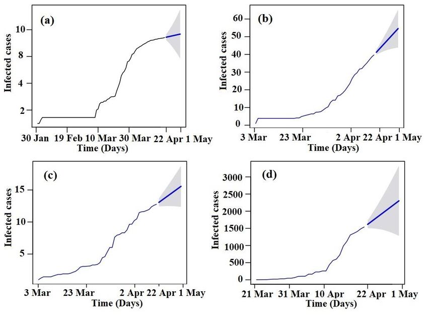
Figure 5: (a) 10-days ahead forecast (22 April to 1 May 2020) using Holt's Method
for Kerala; (b) 10-days ahead forecast (22 April to 1 May 2020) using Holt's Method
for Rajasthan; (c) 10-days ahead forecast (22 April to 1 May 2020) using Holt's
Method for Delhi; (d) 10-days ahead forecast (22 April to 1 May 2020) using Holt's
Method for Madhya Pradesh.

Figure 6: (a) 10-days ahead forecast (22 April to 1 May 2020) using Holt's Method
for Tamil Nadu;(b) 10-days ahead forecast (22 April to 1May 2020) using Holt's
Method for Karnataka.

 12

Figure 7: (a)10-days ahead forecast (22 April to 1 May 2020) using Holt's Method
 for Uttar Pradesh; (b) 10-days ahead forecast (22 April to 1 May 2020) using Holt's
 Method for Telangana.

Figure 8:(a) 10-days ahead forecast (22 April to 1 May 2020) using ARIMA(2,1,0) model
for Kerala; (b) 10-days ahead forecast (22 April to 1 May 2020) using ARIMA(0,1,1)
model for Rajasthan; (c) 10-days ahead forecast (22 April to 1 May 2020) using
ARIMA(1,1,2) model for Delhi; (d) 10-days ahead forecast (22 April to 1 May 2020) using
ARIMA(0,1,1) model for Madhya Pradesh.

 13

Figure 9:(a) 10-days ahead forecast (22 April to 1 May 2020) using ARIMA(2,1,1) model
for Uttar Pradesh; (b) 10-days ahead forecast (22 April to 1 May 2020) using ARIMA(2,1,0)
model for Telangana; (c) 10-days ahead forecast (22 April to 1 May 2020) using
ARIMA(1,1,1) model for Tamil Nadu; (d) 10-days ahead forecast (22 April to 1 May 2020)
using ARIMA(3,1,0) model for Karnataka.

 Figure 10: (a) 10-days ahead forecast (22 April to 1 May 2020) using
 ARIMA(0,1,0) model for Gujarat; (b) 10-days ahead forecast (22 April to 1
 May 2020) using ARIMA(0,1,2) model for Maharashtra.

 14

Figure 11: (a) 10-days ahead forecast (22 April to 1 May 2020) using Holt's Method for
 Gujarat; (b) 10-days ahead forecast (22 April to 1 May 2020) using Holt's Method for
 Maharashtra.

Figure 12:Spatial distribution of the coronavirus outbreak in the period of 30 Jan to 1 April
2020.

 15

Figure 13:Spatial distribution of the coronavirus outbreak in the period of 30 Jan to 1 May 2020.

5 Data Availability

We obtained daily updates of the cumulative number of infected cases and deaths of the corona-virus
illness for India from Worldometer website (online available:
https://www.worldometers.info/corona-virus/country/india/). To obtain the state-wise cumulative
number of infected cases and deaths for the corona-virus illness we used the government of India
website (online available: https://www.mygov.in/corona-data/covid19-statewise-status). We
gathered data of infected case(s) every day at 12 midnight (GMT-5) from 30 January to 21 April
2020. And forecasted the cumulative number of infected cases and deaths of the epidemic over the
India and the cumulative number of infected cases in ten Indian states: Kerala, Maharashtra, Delhi,
Gujarat, Tamil Nadu, Telangana, Uttar Pradesh, Madhya Pradesh, Karnataka, and Rajasthan, which
show a high burden of COVID-19 cases.

6 Conflicts of Interest
The authors declare no conflicts of interest.

7 FundingStatement
Research Support is provided by the Indian Institute of Technology Mandi.

References

[1]Roosa, K., Lee, Y., Luo, R., Kirpich, A., Rothenberg, R., Hyman, J.M., Yan, P. and Chowell, G.,
2020. Short-term Forecasts of the COVID-19 Epidemic in Guangdong and Zhejiang, China: February
13–23, 2020. Journal of Clinical Medicine, 9(2), p.596.

[2]Elmousalami, H.H. and Hassanien, A.E., 2020. Day Level Forecasting for corona-virus Disease
(COVID-19) Spread: Analysis, Modeling and Recommendations. arXiv preprint arXiv:2003.07778.

 16

[3] Luz, P.M., Mendes, B.V., Codeço, C.T., Struchiner, C.J. and Galvani, A.P., 2008. Time series
analysis of dengue incidence in Rio de Januaryeiro, Brazil. The American journal of tropical medicine
and hygiene, 79(6), pp.933-939.

[4]Wongkoon, S., Jaroensutasinee, M. and Jaroensutasinee, K., 2012. Development of temporal
modeling for prediction of dengue infection in Northeastern Thailand. Asian Pacific journal of
tropical medicine, 5(3), pp.249-252.

[5] Liu, Q., Liu, X., Jiang, B. and Yang, W., 2011. Forecasting incidence of hemorrhagic fever with
renal syndrome in China using ARIMA model. BMC infectious diseases, 11(1), p.218.

[6] Rios, M., Garcia, J.M., Sanchez, J.A. and Perez, D., 2000. A statistical analysis of the seasonality
in pulmonary tuberculosis. European journal of epidemiology, 16(5), pp.483-488.

[7]ABenvenuto, D., Giovanetti, M., Vassallo, L., Angeletti, S. and Ciccozzi, M., 2020. Application of
the ARIMA model on the COVID-2019 epidemic dataset. Data in brief, p.105340.

[8] Zhang, Y., Yang, H., Cui, H. and Chen, Q., 2019. Comparison of the Ability of ARIMA, WNN
and SVM Models for Drought Forecasting in the Sanjiang Plain, China. Natural Resources Research,
pp.1-18.

[9]Supriatna, A., Susanti, D. and Hertini, E., 2017, January. Application of Holt exponential
smoothing and ARIMA method for data population in West Java. In IOP Conference Series:
Materials Science and Engineering (Vol. 166, No. 1, p. 012034). IOP Publishing.

[10] Jere, S. and Siyanga, M., 2016. Forecasting inflation rate of Zambia using Holt’s exponential
smoothing. Open journal of Statistics, 6(2), pp.363-372.

[11] Shi, Y.P. and Ma, J.Q., 2010. Application of exponential smoothing method in prediction and
warning of epidemic mumps. Zhongguoyimiao he mianyi, 16(3), pp.233-237.

[12] Gupta, R. and Pal, S.K., 2020. Trend Analysis and Forecasting of COVID-19 outbreak in India.
medRxiv.

[13]Roosa, K., Lee, Y., Luo, R., Kirpich, A., Rothenberg, R., Hyman, J.M., Yan, P. and Chowell, G.,
2020. Real-time forecasts of the COVID-19 epidemic in China from February 5th to February 24th,
2020. Infectious Disease Modelling, 5, pp.256-263.

[14] Singh, R. and Adhikari, R., 2020. Age-structured impact of social distancing on the COVID-19
epidemic in India. arXiv preprint arXiv:2003.12055.

[15] Liu, Z., Magal, P., Seydi, O. and Webb, G., 2020. Predicting the cumulative number of cases for
the COVID-19 epidemic in China from early data. arXiv preprint arXiv:2002.12298.

[16] Liu, Z., Magal, P., Seydi, O. and Webb, G., 2020. Predicting the cumulative number of cases for
the COVID-19 epidemic in China from early data. arXiv preprint arXiv:2002.12298.

[17] Tariq, A., Lee, Y., Roosa, K., Blumberg, S., Yan, P., Ma, S. and Chowell, G., 2020. Real-time
monitoring the transmission potential of COVID-19 in Singapore, February 2020. medRxiv.

[18] Box, G.E., Jenkins, G.M., Reinsel, G.C. and Ljung, G.M., 2015. Time series analysis: forecasting
and control. John Wiley & Sons.

 17

[19] Kwiatkowski, D., Phillips, P.C., Schmidt, P. and Shin, Y., 1992. Testing the null hypothesis of
stationarity against the alternative of a unit root. Journal of econometrics, 54(1-3), pp.159-178.

[20] Said, S.E. and Dickey, D.A., 1984. Testing for unit roots in autoregressive-moving average
models of unknown order. Biometrika, 71(3), pp.599-607.

 18