A Novel Fading Memory Square Root UKF Algorithm for the High-precision State of Charge Estimation of High-power Lithium-ion Batteries
←
→
Page content transcription
If your browser does not render page correctly, please read the page content below
Int. J. Electrochem. Sci., 16 (2021) Article ID: 210737, doi: 10.20964/2021.07.68

                                                                           International Journal of
                                                                           ELECTROCHEMICAL
                                                                                   SCIENCE
                                                                                  www.electrochemsci.org

A Novel Fading Memory Square Root UKF Algorithm for the
High-precision State of Charge Estimation of High-power
Lithium-ion Batteries
Weikang Ji, Shunli Wang*, Chuanyun Zou, Haotian Shi

School of information engineering, Southwest University of science and technology, Mianyang,
Sichuan 621010)
*
 E-mail: 497420789@qq.com

Received: 2 March 2021 / Accepted: 8 May 2021 / Published: 31 May 2021

The state-of-charge (SOC) is used to characterize the remaining capacity of power lithium-ion battery.
Using the simplicity of Thevenin equivalent circuit model, a bidirectional online improvement model
that distinguishes the charging and discharging process is proposed to characterize the state of lithium-
ion batteries, and the on-line parameter identification of the model is carried out by using the least square
method of evolving memory. A novel square root unscented Kalman iterative algorithm based on the
dynamic state-of -charge of the lithium battery is designed, and the SOC estimation effect of the
combined dynamic estimation algorithm and the unscented Kalman algorithm (UKF) is compared. The
dynamic stress test mode (DST) experiment was carried out on the ternary lithium-ion battery at 25℃.
The simulation results show that the average error of the lithium-ion battery SOC estimation of the
dynamic joint estimation algorithm and the unscented Kalman algorithm are 1.23% and 2.11%
respectively. The experimental results show that the joint algorithm based on the square root unscented
Kalman algorithm and the fading memory method has better tracking effect, and has higher SOC
estimation accuracy and stability.

Keywords: lithium-ion battery; Fading memory algorithm; state of charge; Square Root Unscented
Kalman filter algorithm; dynamic stress test.

1. INTRODUCTION

        At present, with the rapid economic development, the pollution and transportation problems
facing the world are becoming more and more serious [1]. The energy crisis caused by excessive energy
consumption has attracted widespread attention from countries around the world [2]. Therefore, all
countries are committed to the development and development of new energy sources. Research to meet
huge energy demand and alleviate environmental pollution [3]. Among the research results of many new
energy projects, lithium-ion battery (LIB) has received extensive attention and research due to their
Int. J. Electrochem. Sci., 16 (2021) Article ID: 210737 2
advantages such as high energy density , long life, small size, no pollution, no memory effect, and large
output power [4]. Application has become a key project in the field of new energy development, with
broad development prospects [5]. While the lithium-ion battery technology is booming, its state-of-
charge (SOC) and state-of-health (SOH) have become the focus and difficulty of lithium battery
research. For lithium-ion battery, high-accuracy estimation of the state of charge is necessary to give full
play to its performance [6]. It is exactly significant to real-time state detection and safety control of
lithium-ion battery, it also plays a key role in improving the efficiency of the Battery Management
System (BMS) [7]. Because the power lithium battery has strong nonlinearity, its SOC cannot be
obtained directly by sensors or other measurement methods. It must be measured by measuring the
battery voltage, operating current, battery internal resistance and other physical quantities and using
certain mathematical methods to estimate, so that The estimation of the state-of-charge of a lithium
battery needs to rely on the equivalent model established for the characteristics of the lithium battery
[8]. Moreover, due to the strong nonlinear characteristics exhibited by the lithium battery under complex
operating conditions, it is difficult to accurately rely on the equivalent model only, characterize the
characteristics of lithium batteries [9]. The square root unscented Kalman filter (SRUKF) algorithm
improved by the unscented kalman Filter (UKF) algorithm is applied to the process SOC estimation of
lithium batteries [10], and an accurate equivalent circuit model (ECM) is established to improve the
algorithm estimation effect.
In the field of lithium-ion battery state estimation, equivalent modeling is an indispensable step
[11]. The accuracy and stability of the model directly determine the state estimation effect of the lithium-
ion battery [12]. In the process of equivalent modeling, the parameter identification of the model is the
most important link [13]. Least squares method is a commonly used parameter identification. Compared
with artificial neural network (ANN) algorithms and fuzzy logic algorithms [14,15], the principle of least
squares method is simpler and has fewer steps. However, only the least square method cannot meet the
accuracy requirements of parameter identification [16]. Based on the principle of recursive least squares
[17], the method of adding a forgetting factor in the iterative process is called fading memory method
recursive least square (FMRLS). The advantage of this method is that it can continuously increase the
weight of new data and continuously optimize the lithium battery model to improve the model The
accuracy and anti-interference ability [18]. Through the capacity and hybrid pulse power characteristic
(HPPC) [19] experiments on the battery at different temperatures, and analyzing the open circuit voltage,
ohmic internal resistance [20] and polarization resistance of LIB at different temperatures, the battery
characteristics and state of charge [21] can be obtained. The parameters of LIB model are identified by
fading memory recursive least square method.
Based on the fading memory method and the square root unscented Kalman algorithm, a joint
iterative algorithm for lithium battery SOC estimation is proposed. Through forgetting factor [22] and
Kalman gain [23], online lithium battery equivalent modeling and SOC estimation are realized. At the
same time, the iterative process is optimized to reduce the amount of calculation.Int. J. Electrochem. Sci., 16 (2021) Article ID: 210737 3
2. MATHEMATICAL ANALYSIS
2.1 Process distinguished online equivalent circuit modeling
In the process of SOC estimation of lithium battery, it is very important to establish the battery
equivalent model to simulate the working state and Internal characteristics of batteries. The estimation
accuracy of SOC largely depends on the degree of characterization of the dynamic characteristics of the
battery by the equivalent model [24]. Thevenin model is composed of a parallel RC circuit of internal
resistance model, which has the advantages of simple principle and few parameters [25]. Moreover, the
RC circuit in the model can better simulate the polarization effect in the process of battery charging and
discharging, and characterize the internal chemical reaction of battery [26]. Thevenin model is one of
the common equivalent circuit models, On the basis of Thevenin model, considering the different battery
characteristics of lithium-ion batteries during charging and discharging, the internal resistance of the
model is divided into equivalent resistances under different working conditions, so as to optimize the
model and make it more effective to characterize the working process of lithium-ion batteries [27]. The
Schematic diagram of the improved model is shown in Figure 1.
U1
R1
D1 Rp
R2 +
UOC Cp
D2
Udis Ucha RO
UL
-
I1 IL
I2
Figure 1. Improved equivalent circuit model
In Figure 1, UOC is the open circuit voltage, UL is the circuit terminal voltage, R1 and R2 are the
ohmic internal resistance during battery discharging and charging, namely Ro under different working
conditions. RP is the polarization resistance, and CP is the polarization capacitance. Ro reflects the
transient change of the battery terminal voltage at the beginning and end of discharge of the lithium
battery [28]. The parallel circuit of RP and CP characterizes the polarization effect during battery charging
and discharging. The circuit equation can be obtained from the circuit model in the figure:
U L U OC U P I L R0
dU P U p (1)
I L CP dt R
P
Corresponding to Figure 1, the current direction when the battery is discharged is positive, and
the current direction is negative when the battery is charged. UP(0) is used to represent the initial voltageInt. J. Electrochem. Sci., 16 (2021) Article ID: 210737 4
of the battery polarization process, and the time domain relationship equation of Thevenin equivalent
circuit model as shown in equation (2) can be established according =RPCP.
( t / )
U P (t ) U P (0) e I L RP (1 e (t / ) )
( t / ) ( t / )
(2)
L
U (t ) U oc U P (0) e I L (t ) R0 I L RP (1 e )
2.2 Model optimization of fading memory method
The fading memory method is a parameter identification method based on recursive least square
method. By adding forgetting factor, the proportion of new data is continuously increased, so as to
optimize and update the model.
First of all, from the basic principle of the least squares method [29], the system error square sum
is minimized, the parameter matrix is derivated, and the parameter matrix is replaced with the system
input and output matrix x, y, the basic parameter identification formula of the least square method can
be obtained:
y (k ) x(k )T (k )
ˆ (3)
( X X ) X Y
T 1 T
According to the principle formula in Eq. (2), the iterative formula of the recursive least square
method can be obtained:
ˆN 1 ( X N 1T X N 1 )1 X N 1T YN 1
XN YN (4)
X N 1 , YN 1
x( N 1) y ( N 1)
On the basis of the recursive least squares method, a forgetting factor is added to the input and
output recursive links to increase the weight of subsequent data.
XN YN
X N 1, , YN 1, (5)
x( N 1) y ( N 1)
After obtaining the input and output matrix with forgetting factor, use the principle of recursive
least squares to derive, and get the recursive formula of the iterative algorithm for parameter
identification of the fading memory method:
PN ( X T X ) 1
( N 1) 1/ x ( N 1) PN x( N 1)
T
(6)
P N 1
PN ( N 1) PN x ( N 1) x T
( N 1) PN
/
ˆ ˆ ˆ
N 1 N ( N 1) PN x( N 1) y ( N 1) x ( N 1) N
T
Compared with the recursive least squares method, the fading memory method has the advantage
that by adding the forgetting factor, the gain is constantly updated in the time domain, so that the model
is optimized in real time and can more accurately adapt to the variability of the lithium battery working
environment. The algorithm structure diagram is as follows:Int. J. Electrochem. Sci., 16 (2021) Article ID: 210737 5
FMLRS model parameter identification flowchart
Lithium-ion battery SOC-OCV Verification result
4.5
calibration
Input data
Curve fitting 0.33C 4.2 Us
Ut
1C
OCV (V)
4.0
4.0 2c 3.9
3.8
3.9 3.7
U(V)
3.6
9000 10000 11000 12000 13000
Voltage Current Temperature 3.5
3.6
3.0
0.0 0.2 0.4 0.6 0.8 1.0
SOC(1) 3.3
0 6000 12000 18000 24000
t(s)
Iterative calculation
Comparative
0.15
verification error
0.10
Battery model
U1 0.05
error(1)
ˆN 1 ˆN (N 1)PN x(N 1) y(N 1) xT (N 1)ˆN
R1
D1 Rp 0.00
R2 +
-0.05
UOC Cp
D2
PN 1 PN (N 1)PN x(N 1)x (N 1)PN /
T RO
Udis Ucha UL -0.10
Result
(N 1) 1/ x (N 1)PN x(N 1)
T I1 IL
- -0.15
0 6000 12000 18000 24000
t(s)
I2
Figure 2. Structure diagram of fading memory algorithm
2.3 Square unscented Kalman iterative calculation
At present, the commonly used methods for estimating the battery state of charge include the
following methods: ampere-hour integration method, open circuit voltage method, and Kalman filter
method [30]. Among them, the open circuit voltage method cannot realize the real-time online estimation
of the battery SOC; although the ampere-hour integration method can meet the requirements of real-time
SOC estimation, it is not suitable for high-precision SOC because the calculation process is prone to
large cumulative errors. Estimation occasions; Kalman filter method, which can estimate the SOC value
in real time and has high estimation accuracy, has become the current research hotspot of SOC
estimation. The Kalman filter algorithm is a filter theory (Kalman Filter, KF) created by the state space
theory in the time domain. The core idea of the algorithm is to make an optimal state estimation of the
system which is with dynamic characteristic in the sense of least mean square[31]. The algorithm system
of "prediction-estimation-prediction" improves the accuracy of system estimation. However, the Kalman
filter algorithm is only suitable for linear systems. During the working process of lithium batteries, most
of them exhibit nonlinear characteristics. Therefore, the application of the Kalman filter algorithm must
first linearize the nonlinear system, which will introduce errors.
The Square Root Unscented Kalman Filter (SR-UKF) is an improved algorithm based on the
Unscented Kalman Filter (UKF) [32]. Like the Unscented Kalman Filter, it eliminates the need for
nonlinearity. The method of linearizing the function directly deals with the nonlinear system. The biggest
difference between it and the unscented Kalman algorithm is that the SR-UKF algorithm uses the square
root of the error covariance of the state variable to replace the error covariance of the state variable, and
directly transmits the square root of the covariance value to avoid the problem of Re-decompose [33].
The advantages of this method are it ensures the positive semi-definiteness and numerical stability of
the state variable covariance matrix, Moreover, it can overcome the filtering divergence [34]. ComparedInt. J. Electrochem. Sci., 16 (2021) Article ID: 210737 6
with UKF, SR-UKF has higher accuracy and anti-interference in lithium battery SOC estimation. The
flow chart of the SR-UKF algorithm is shown in Figure 3.
Square root unscented Kalman algorithm
Cholesky factor Efficient least
QR decompose
updating square method
Reprediction
Initial value of k
Status update
initialization
determination
Update
k-1
Sigma point
Time update
acquisition
Forecast
Figure 3. SR-UKF Algorithm structure diagram
Error! Reference source not found.
The square root unscented Kalman algorithm uses three powerful linear algebra techniques,
namely QR decomposition, Cholesky factor update and efficient least squares [35]. The specific
algorithm mainly consists of four parts, which are respectively named initialization, sigma point
acquisition, time update and status update.
(1) Initialization:
Determine the initial value of the state variable and the initial value P0 of the error covariance.
S0 is the cholesky decomposition factor of the covariance P0. The initial value is determined as shown
in Eq. (4).
xˆ0 E x0
P0 E x0 xˆ0 x0 xˆ0
T
(7)
S0 chol P0
(2) Sigma point collection:
xk 1 xˆk 1 , i 0
i
i
xk 1 xˆk 1 n Sk 1 , i 1 ~ n
i
(8)
i
xk 1 xˆk 1 n Sk 1 , i n 1 ~ 2n
i n
Int. J. Electrochem. Sci., 16 (2021) Article ID: 210737 7
Ski represents the ith column of the Cholesky factor of the state variable covariance at time k.
The calculation of the mean weight ωm and the variance weight ωc is consistent with the unscented
Kalman algorithm.
(3) Time update:
On the basis of obtaining the value of the state variable and input variable at k-1 time, one-step
prediction of the state variable is made through the state equation.
xki |k 1 f xki 1|k 1 , uk 1
2n (9)
xˆk |k 1 m xk |k 1
i i
i 0
Taking the one-step prediction of sampling points into account, QR decomposition of the error
covariance of the state variable is carried out, considering that the different values of α and k may cause
the negative value of ωc0, so Eq. (10) is used to ensure the matrix Positive semi-definite, Sxk represents
the square root update value of the state variable error covariance at time k [36].
xk
S qr 1:2 n x1:2 n xˆ
c k |k 1 k |k 1
, Qk
(10)
S xk cholupdate S xk , abs c0 xk0|k 1 xˆk |k 1 , sign c0
According to the one-step prediction result of the state variable in Eq. (9), the one-step prediction
value of the observed variable obtained from the observation equation is as follows. Syk represents the
square root update value of the error covariance of the observed variable at time k
yki |k 1 h xki |k 1 , uk
2n
k |k 1 m yk |k 1
ˆ i i
y
i 0
(11)
S yk qr c1:2 n y1:2 n
ˆ
x k |k 1 , R
k |k 1 k
0 0
S yk cholupdate S yk , abs c yk |k 1 yˆ k |k 1 , sign c
0
(4) Status update
The cross-covariance between the state variable and the observed variable will directly affect the
size of the Kalman gain, and the accuracy of the Kalman gain will affect the estimation effect of the
SOC. The calculation formulas of cross-covariance and Kalman gain are shown in Eq. (12). The system
state variable update and error covariance update are shown in equation (16), where yk is the
experimental measurement value at time k.
2n
xy ,k c xk |k 1 xˆk |k 1 yk |k 1 yˆ k |k 1
T
P i i i
i 0 (12)
xy , k S yk S yk
K P T 1
k
The system state variable update and error covariance update are shown in equation (16), where
yk is the experimental measurement value at time k.Int. J. Electrochem. Sci., 16 (2021) Article ID: 210737 8
xˆk |k xˆk |k 1 K k yk yˆ k |k 1
(13)
Sk cholupdate S xk , K k S yk , 1
In the SR-UKF algorithm, through a Cholesky factorization, the filter is initialized by calculating
the square root of the state variable covariance matrix. However, in subsequent iterations, the spread and
updated Cholesky factor directly formed the sigma point. The time update Sxk of the Cholesky factor is
calculated using the QR decomposition of the composite matrix containing the weighted propagation
sigma points plus the square root of the process noise covariance matrix, and the subsequent Cholesky
update is essential. These two steps replace the time update of Px,k|k-1 in the covariance update of state
variables, overcome the shortcomings of poor stability of the UKF algorithm, and ensure the positive
semi-definiteness of the covariance matrix.
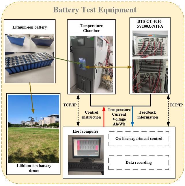
3. EXPERIMENTAL ANALYSIS
Choose the ternary lithium-ion battery for discharge experiment. The rated capacity of the battery
is 70Ah. The instruments used in the test include a high-power battery charge and discharge tester, a
three-layer independent temperature-controlled laboratory (BTT-331C) and other auxiliary experimental
equipment. Considering the influence of temperature changes of model parameters, experiments were
carried out at multiple different temperatures. The test equipment is shown in Fig.4.
Figure 4. The experiments equipmentInt. J. Electrochem. Sci., 16 (2021) Article ID: 210737 9
3.1 OCV-SOC relationship curve fitting
In the process of using the FMRLS method to identify the parameters of the lithium-ion battery
online model, the SOC and OCV of the battery will be iteratively calculated as variables in the state
space equation. In the process of estimating the parameters, the difference between SOC and OCV The
functional relationship is one of the necessary initial information [37], and an accurate OCV-SOC
relationship curve is the key to improving the accuracy of model parameter identification according to
the experiment results in literature [38]. Considering the influence of temperature on the working status
of lithium-ion batteries, the experiment was carried out under different temperature conditions to
improve the dynamic stability of the model and explore ways to improve the accuracy of online
parameter identification.
Before performing various tests on the lithium battery, it is necessary to calibrate its capacity
first to obtain its nominal capacity information. The specific calibration method steps are as follows:
(1) The battery is charged at a constant current rate of 1 C, and the charging cut-off voltage
is set to 4.2V. Then it is converted to constant voltage charging. The charging cut-off current is 0.02C
to ensure that the battery is saturated.
(2) In order to obtain a stable battery voltage, the battery is shelved after charging. Because
of the capacity of the selected lithium battery, the settling time is set to 40 minutes.
(3) The battery discharges at a constant current rate of 1 C and reaches the cut-off voltage of
2.5V.
After calibrating the capacity of the lithium-ion battery, conduct a fixed-stage discharge
experiment at different rates. Taking into account the impact of discharge rate on the discharge efficiency
of lithium-ion batteries, a fixed-stage charge and discharge experiment under different charge and
discharge rates was carried out to explore ways to improve the accuracy of OCV-SOC calibration. The
specific test method is as follows:
1) Charge the lithium-ion battery with constant current, and judge whether it reaches the full
state according to whether the segment voltage reaches 4.2V. After charging is complete, set the lithium-
ion battery for 40 minutes.
2) Discharge the lithium battery at a specific rate. After the discharge capacity reaches 10%
of the total capacity, the lithium battery is set for 10 minutes.
3) After each discharge, detect the voltage of the lithium-ion battery segment, if the segment
voltage reaches 2.5V, stop the discharge.
The charging process of a lithium ion battery has the opposite judgment conditions for the
discharge process, and the test process is the same. The flow chart of the charge and discharge test
method is as follows:Int. J. Electrochem. Sci., 16 (2021) Article ID: 210737 10
Start Start
N Y N Y
battery battery
U=4.2? U=2.5?
charging discharging
Y N Y N
End SOC=0? End SOC=1?
Set for 10min Set for 10min
NC current discharge NC current charge
Set for 40min Set for 40min
10% 10%
(a) Discharging process (b) Charging process
Figure 5. OCV-SOC calibration experiment flow chart
After calibrating the capacity of the lithium-ion battery, the nominal capacity of the battery is
70.21Ah. Under the temperature condition of 25℃, the battery is subjected to a fixed-stage discharge
test. Discharge the battery with constant current at 0.33C, 1C, 2C discharge rates, record the open circuit
voltage of the battery at a specific SOC node, and obtain a continuous OCV-SOC relationship curve
through curve fitting according to the discrete relationship between open circuit voltage and state of
charge, According to the curve relationship, use the least square method to simulate the discharge voltage
of the lithium battery, and compare it with the experimental test voltage to find the optimal discharge
rate. The figure below shows the comparison between the fitted curve and the simulation results and
errors.
4.2
4.2 0.33C real
1c
1C 4.1
OCV (V)
0.33c
3.9 2c
U (V)
2c
4.0
3.6
3.5283 3.9
3.5463
3.3 3.4753
3.8
0.2 0.4 0.6 0.8 1.0 0 1000 2000 3000 4000
SOC(1) t (s)
A. OCV-SOC fitting curve B. BBDST operating condition simulation curveInt. J. Electrochem. Sci., 16 (2021) Article ID: 210737 11
4.15 0.04
real
1c Err
1c
0.33c Err
4.10 0.33c 0.02 2c Err
2c
U (V)
Err
4.05
0.00
4.00
-0.02
3.95
-0.04
900 1200 1500 1800 2100 2400 0 1000 2000 3000 4000
t (s) t (s)
C. Partial enlarged view of simulation curve D. Simulation error comparison curve
Figure 6. Comparison results of simulation and experiment
It can be seen from the experimental results that, as verified by B.Ng, M.O and others in the
literature [39-40], under the same temperature conditions, appropriately reducing the discharge rate of
lithium-ion batteries can improve their discharge efficiency, and help establish a more accurate SOC-
OCV relationship.
3.2 Online parameter identification
For the purpose of verifying the on-line identification efficiency of the algorithm, the dynamic
stress test of lithium-ion battery is carried out. The parameters in the equivalent circuit model of lithium
battery are identified by the voltage and current obtained. After the results are obtained, the real-time
estimated values of each parameter are added into the circuit model to obtain the simulation voltage. The
accuracy of parameter identification is verified by comparing simulation voltage with test voltage.
To verify the effectiveness and generality of the limited memory method, the lithium battery was
tested under HPPC condition and DST condition, and the experimental results were compared with the
identification simulation results, and the voltage curve comparison results were shown in Fig.7 and Fig.8.
4.5 0.02
Us
Ut 0.01
4.0
U (V)
Err
0.00
3.5 -0.01
-0.02
3.0
0 6000 12000 18000 24000 0 6000 12000 18000 24000
t (s) t (s)
(a) Real value and predicted value of SOC (b) SOC prediction error(DST)
Figure 7. Comparison and error diagram under HPPC conditionInt. J. Electrochem. Sci., 16 (2021) Article ID: 210737 12
0.15
4.2 Us
Ut error
4.0 0.10
3.9
3.8
3.9 3.7 0.05
error(1)
U(V)
3.6
9000 10000 11000 12000 13000
0.00
3.6
-0.05
-0.10
3.3
0 6000 12000 18000 24000 -0.15
0 6000 12000 18000 24000
t(s)
t(s)
(a) Real value and predicted value of SOC (b) SOC prediction error(DST)
Figure 8. Comparison and error diagram under DST condition
It can be seen from the results that the least square on-line parameter identification method has a
good identification effect. In the HPPC operating condition where the experimental curve is relatively
smooth, the average error between the model simulation voltage and the experimental voltage is only
1.37%,Compared with the offline identification method proposed by Ng in literature [41], this algorithm
increased the accuracy by about 0.5% under the same experimental conditions. And the online
identification method is more real-time and authentic.
In the DST operating condition where the experimental voltage curve is more complicated, the
average error between the model simulation voltage and the experimental voltage is only 2.56 %.
Moreover, It can be seen from the comparison error that in the process of model characterization, the
simulation curve has no obvious jump compared to the experimental curve, and the maximum error is
within a reasonable range, which effectively improves the stability and robustness of the
model.Compared with the improved online identification method of PNGV model proposed by Xie in
literature [42], this method has a simpler model and a more stable identification process.
3.3 SOC estimation accuracy verification under multiple working conditions
Dynamic stress test (DST) is a kind of complex working condition after the simplification of
urban operation condition in the United States, which plays an important role in verifying the SOC
estimation effect of the algorithm [43]. In order to further test the SOC estimation accuracy of SR-UKF
algorithm, DST condition test is carried out for ternary lithium battery with rated capacity of 70ah at 25
℃, SOC value of lithium battery is estimated by using model and algorithm, and the estimation results
of UKF algorithm and SR-UKF algorithm under the same conditions are compared, as shown in Fig.9
(a), and Figure 8 (b) is the estimation error comparison of the two algorithms.Int. J. Electrochem. Sci., 16 (2021) Article ID: 210737 13
1.00 SOC real UKF error
UKF prediction 0.015 SR-UKF error
SR-UKF prediction
0.75
SOC
0.010
Err
0.50 0.375
u(v)
0.300
0.005
0.25 0.225
4000 4400 4800
t(s)
0.000
0.00
0 1500 3000 4500 0 1500 3000 4500
t(s) t(s)
(a) Comparison curve of SOC prediction under (b) Prediction error comparison curve
DST condition
Figure 9. Comparison of SOC estimation results of DST algorithm
As is shown in Fig.9. The SR-UKF algorithm has a greater improvement in the SOC estimation
accuracy than the UKF algorithm. The experimental results show that under DST condition, SR-UKF
algorithm has a high accuracy in estimating SOC value of lithium battery, and the estimation error is
stable within 0.58%. However, it fails to judge whether the estimation error of the algorithm stabilizes
over time according to the curve in the figure.
As mentioned in literature [44], the BBDST (Beijing Bus Dynamic Stress Test) operating
condition and HPPC (Hybrid Pulse Power Characteristic) condition can more accurately test the stability
and anti-interference of the state estimation of lithium-ion batteries by analyzing the characteristics of
the battery and electric vehicle operating conditions. To further verify the accuracy and stability of the
SOC estimation of the SR-UKF algorithm, the BBDST and HPPC condition were used to compare the
actual SOC value of the lithium-ion battery with the estimated simulated SOC value. The results are
shown in Fig.10 and Fig.11.
1.0 Test 0.02
UKF
0.8 0.01
SR-UKF
SOC
Err
0.6 0.60
0.55
0.00
0.4 0.50
0.45
0.40 -0.01 UKF
0.35
0.2 0.30
16000 18000 20000 22000 24000
-0.02 SR-UKF
0.0
0 6000 12000 18000 24000 30000 0 6000 12000 18000 24000 30000
t (s) t (s)
(a) SOC comparison curve (b) Estimated error comparison curve
Figure 10. SOC estimation result under BBDST conditionInt. J. Electrochem. Sci., 16 (2021) Article ID: 210737 14
1.0 Test 0.03 Err-UKF
0.8 UKF 0.02 Err-SR-UKF
SR-UKF
0.01
SOC
0.6
Err
0.4 0.00
-0.01
0.2
-0.02
0.0
-0.03
0 6000 12000 18000 24000 0 6000 12000 18000 24000
t (s) t (s)
(a) SOC comparison curve (b) Estimated error comparison curve
Figure 11. SOC estimation result under HPPC condition
As is shown in Fig.10 and Fig.11. SR-UKF algorithm not only has the advantages of reducing
the calculation amount, but also has a more effective processing of non-linear characteristics of lithium
battery at the beginning and end of discharge, and has a higher SOC estimation accuracy. In more
complex BBDST conditions, the SOC estimation error of the SR-UKF algorithm remains at about
1.46%, compared with EKF algorithm mentioned in literature [45],under the same experimental
conditions and experimental temperature conditions, its lithium battery SOC estimation accuracy is
2.16%, indicating that SR-UKF algorithm has better stability and robustness. The improvement value of
the algorithm is verified, which has a certain significance for the estimation of the state of charge of
lithium battery.
The online lithium-ion battery identification model obtained by using the least squares of the
fading memory method is in good agreement with the SR-UKF algorithm. In the BBDST experiment,
the error between the SOC curve of the lithium ion battery obtained by the algorithm simulation and the
SOC curve of the lithium ion battery obtained according to the real experimental data is only 0.91%; in
the HPPC experiment, the difference between the simulated SOC curve and the real SOC curve The
error is only 0.94%. Compared with the UKF algorithm [46-47], the SR-UKF algorithm not only greatly
improves the accuracy of lithium-ion battery SOC estimation, but also greatly improves the stability and
robustness of the estimation, making the entire simulation process more stable and smooth.
4. CONCLUSIONS
In order to accurately estimate the SOC of lithium battery, the equivalent circuit model is used
to characterize the characteristics of lithium battery and simulate its working state. The current and
voltage data in the state of battery charge and discharge are obtained by HPPC experiment. The SOC
value of lithium battery is calculated according to the definition. The function relationship between SOC
and the parameters in the equivalent model is established by curve fitting method. Comparing the voltage
estimation curve with the real voltage curve, the model identification accuracy is within 1.1%. ComparedInt. J. Electrochem. Sci., 16 (2021) Article ID: 210737 15
with the second-order Thevenin model and its parameter identification method proposed in Literature 1,
it simplifies the model identification workload and improves about 0.4% in terms of the model
representation accuracy. Meanwhile, the characterization of the charging and discharging process of
lithium batteries is more targeted.
The SOC estimation accuracy of the square root unscented Kalman filter (SR-UKF) algorithm
was verified by Dynamic Stress Test (DST), Beijing Bus Dynamic Stress Test(BBDST) and Hybrid
Pulse Power Characteristic (HPPC) test. The prediction errors are all within 1%. The adaptive Kalman
filter estimation method mentioned in literature [47] achieves the fast convergence of the estimation of
the state of charge of lithium batteries through an improved adaptive factor; the improved extended
Kalman filtering estimation method proposed in literature [48] reduces the iterative calculation process
of the internal parameters of the lithium battery model by removing the redundant Taylor expansion, and
improves the estimation speed. Compared with the above algorithm, the proposed algorithm in this
article greatly improves the stability and robustness of the estimation, reduces the sudden change caused
by noise during the estimation of the lithium-ion SOC, and improves the estimation accuracy of the
lithium-ion battery state of charge by 0.4%~0.6 %, and to a certain extent improve the stability of the
energy supply of lithium-ion batteries. It provides an improved idea for the lithium battery SOC
estimation algorithm, which has certain research significance.
ACKNOWLEDGEMENTS
The work is supported by the National Natural Science Foundation of China (No. 61801407), Natural
Science Foundation of Southwest University of Science and Technology (No.17zx7110, 18zx7145), Si
chuan science and technology program (No. 2019YFG0427), China Scholarship Council (No. 2019085
15099), and Fund of Robot Technology Used for Special Environment Key Laboratory of Sichuan Pro
vince (No. 18kftk03).
References
1. M. Al-Gabalawy, N. S. Hosny, J. A. Dawson and A. I. Omar, International Journal Of Energy
Research, 45 (2021) 6708.
2. L.-Z. Deng, F. Wu, X.-G. Gao and W.-p. Wu, Rare Metals, 39 (2020) 1457.
3. Z. E, H. Guo, G. Yan, J. Wang, R. Feng, Z. Wang and X. Li, Journal Of Energy Chemistry, 55
(2021) 524.
4. G. Dong, F. Yang, K.-L. Tsui and C. Zou, Ieee Transactions on Industrial Informatics, 17 (2021)
2587.
5. K. Eguchi, A. Shibata, W. Do and F. Asadi, Energy Reports, 6 (2020) 1151.
6. M. Faisal, M. A. Hannan, P. J. Ker, M. S. Abd Rahman, R. A. Begum and T. M. I. Mahlia, Energy
Reports, 6 (2020) 215.
7. Y. He, Q. Li, X. Zheng and X. Liu, Journal Of Power Electronics, 21 (2021) 590.
8. Z. He, Z. Yang, X. Cui and E. Li, Ieee Transactions on Vehicular Technology, 69 (2020) 14618.
9. L. Jiang, Y. Huang, Y. Li, J. Yu, X. Qiao, C. Huang and Y. Cao, Ieee Transactions on Intelligent
Transportation Systems, 22 (2021) 622.
10. A. A. Kamel, H. Rezk and M. A. Abdelkareem, International Journal Of Hydrogen Energy, 46
(2021) 6061.
11. E. D. Kostopoulos, G. C. Spyropoulos and J. K. Kaldellis, Energy Reports, 6 (2020) 418.Int. J. Electrochem. Sci., 16 (2021) Article ID: 210737 16
12. Z. Lei, T. Liu, X. Sun, H. Xie and Q. Sun, International Journal Of Energy Research, 45 (2021)
3157.
13. A. Khalid and A. I. Sarwat, Ieee Access, 9 (2021) 39154.
14. A. Nath, R. Gupta, R. Mehta, S. S. Bahga, A. Gupta and S. Bhasin, Ieee Transactions on Vehicular
Technology, 69 (2020) 14701.
15. Z. Ren, C. Du, H. Wang and J. Shao, International Journal Of Electrochemical Science, 15 (2020)
9981.
16. M. Aslam, Complex & Intelligent Systems, 7 (2021) 359.
17. T. Tan, K. Chen, Q. Lin, Y. Jiang, L. Yuan and Z. Zhao, Ieee Transactions on Circuits And Systems
I-Regular Papers, 68 (2021) 1354.
18. S. Yang, S. Zhou, Y. Hua, X. Zhou, X. Liu, Y. Pan, H. Ling and B. Wu, Scientific reports, 11 (2021)
5805.
19. Y. Zheng, Y. Lu, W. Gao, X. Han, X. Feng and M. Ouyang, Ieee Transactions on Industrial
Electronics, 68 (2021) 4373.
20. T. Zhao, Y. Zheng, J. Liu, X. Zhou, Z. Chu and X. Han, International Journal Of Energy Research,
45 (2021) 4155.
21. W. Li, Y. Xie, Y. Zhang, K. Lee, J. Liu, L. Mou, B. Chen and Y. Li, International Journal Of
Energy Research, 45 (2021) 4239.
22. N. Peng, S. Zhang, X. Guo and X. Zhang, International Journal Of Energy Research, 45 (2021)
975.
23. J. Yao, M. Zhang, G. Han, X. Wang, Z. Wang and J. Wang, Ceramics International, 46 (2020)
24155.
24. J. Shen, J. Xiong, X. Shu, G. Li, Y. Zhang, Z. Chen and Y. Liu, International Journal Of Energy
Research, 45 (2021) 5586.
25. H. Shi, S. Wang, C. Fernandez, C. Yu, Y. Fan and W. Cao, International Journal Of
Electrochemical Science, 15 (2020) 12706.
26. D. Wang, L. Zheng, X. Li, G. Du, Y. Feng, L. Jia and Z. Dai, International Journal Of Energy
Research, 44 (2020) 12158.
27. S. Park, J. Ahn, T. Kang, S. Park, Y. Kim, I. Cho and J. Kim, Journal Of Power Electronics, 20
(2020) 1526.
28. X. Xia and L. Tang, International Journal Of Energy Research, 45 (2021) 4410.
29. S. Xie, J. Sun, X. Chen and Y. He, International Journal Of Energy Research, 45 (2021) 5795.
30. N. Yan, H. Zhao, T. Yan and S. Ma, Energy Reports, 6 (2020) 1106.
31. X. Zhang, J. He, J. Zhou, H. Chen, W. Song and D. Fang, Science China-Technological Sciences,
64 (2021) 83.
32. H. Shi, S. Wang, C. Fernandez, C. Yu, Y. Fan and W. Cao, International Journal Of
Electrochemical Science, 15 (2020) 12706.
33. X. Xiong, S.-L. Wang, C. Fernandez, C.-M. Yu, C.-Y. Zou and C. Jiang, International Journal Of
Energy Research, 44 (2020) 11385.
34. X. Zhang, J. He, J. Zhou, H. Chen, W. Song and D. Fang, Science China-Technological Sciences,
64 (2021) 83.
35. S. Zhang, X. Guo and X. Zhang, International Journal Of Hydrogen Energy, 45 (2020) 14156.
36. Y. Liu, J. Li, G. Zhang, B. Hua and N. Xiong, Ieee Access, 9 (2021) 34177.
37. Y. Liu, R. Ma, S. Pang, L. Xu, D. Zhao, J. Wei, Y. Huangfu and F. Gao, Ieee Transactions on
Industry Applications, 57 (2021) 1094.
38. S. Marelli and M. Corno, Ieee Transactions on Control Systems Technology, 29 (2021) 926.
39. B. Ng, E. Faegh, S. Lateef, S. G. Karakalos and W. E. Mustain, Journal Of Materials Chemistry A,
9 (2021) 523.
40. M. O. Qays, Y. Buswig, M. L. Hossain, M. M. Rahman and A. Abu-Siada, Csee Journal Of Power
And Energy Systems, 7 (2021) 86.Int. J. Electrochem. Sci., 16 (2021) Article ID: 210737 17
41. L. Zhang, International Journal Of Low-Carbon Technologies, 15 (2020) 607.
42. Y. Xie, K. Dai, Q. Wang, F. Gu, M. Shui and J. Shu, Physical Chemistry Chemical Physics, 23
(2021) 1750.
43. Z. Zhang, Z. Du, Z. Han, H. Wang and S. Wang, International Journal Of Energy Research, 44
(2020) 11840.
44. G. Sethia, S. K. Nayak and S. Majhi, Ieee Transactions on Circuits And Systems I-Regular Papers,
68 (2021) 1319.
45. J. Sihvo, T. Roinila and D.-I. Stroe, Ieee Transactions on Industrial Electronics, 68 (2021) 4916.
46. N. Shateri, Z. Shi, D. J. Auger and A. Fotouhi, Ieee Transactions on Vehicular Technology, 70
(2021) 212.
47. Y.-D. Yan, K.-Y. Hu and C.-H. Tsai, Ieee Transactions on Industrial Electronics, 67 (2020) 6365
© 2021 The Authors. Published by ESG (www.electrochemsci.org). This article is an open access
article distributed under the terms and conditions of the Creative Commons Attribution license
(http://creativecommons.org/licenses/by/4.0/).You can also read