Electromagnetic Force Analysis of Eccentric Axial Flux Permanent Magnet Machines

Hindawi
Mathematical Problems in Engineering
Volume 2020, Article ID 6194317, 16 pages
https://doi.org/10.1155/2020/6194317

Research Article
Electromagnetic Force Analysis of Eccentric Axial Flux Permanent
Magnet Machines

 Qiaoshan Li , Bingyi Zhang, and Aimin Liu
 School of Electrical Engineering, Shenyang University of Technology, Shenyang 110870, China

 Correspondence should be addressed to Qiaoshan Li; liqiaoshan@sut.edu.cn

 Received 1 February 2020; Accepted 6 April 2020; Published 29 April 2020

 Academic Editor: Andrés Sáez

 Copyright © 2020 Qiaoshan Li et al. This is an open access article distributed under the Creative Commons Attribution License,
 which permits unrestricted use, distribution, and reproduction in any medium, provided the original work is properly cited.

 Based on Schwarz–Christoffel mapping, this paper presents a fast analytical method to analyze the electromagnetic force of
 eccentric axial flux permanent magnet machines, considering static, dynamic, and mixed eccentricities. A quasi-3D model of an
 axial flux permanent magnet machine is established, and the magnetic field is obtained by Schwarz–Christoffel mapping. The
 electromagnetic force density is obtained by the Maxwell stress tensor method, and the electromagnetic force density is used to
 characterize the variation of electromagnetic force. The distribution law of electromagnetic force is investigated. The calculated
 results are verified by the finite element method, which has shown that the method in this paper can be widely used in the analysis
 of axial flux permanent magnet machines.

1. Introduction circuit (EMC) method, finite element method (FEM), and
 analytical method. The FEM is the most accurate one at
Due to high efficiency, compact structure, and good heat present [6–8]. However, because of its structural charac-
dissipation performance, axial flux permanent magnet teristics, AFPM motor needs 3D model analysis. This usually
(AFPM) machines are widely used in electric vehicles, fly- requires a higher configuration of computer, and the so-
wheel energy storage, and other fields [1–3]. Because of the lution time is too long, which is disadvantageous in the early
unique structural characteristics of an AFPM machine, the stage of motor design.
eccentricity of a stator and rotor is easy to occur in the The accuracy of the EMC method depends directly on
assembly process, which will bring adverse effects. Therefore, the rationality of the establishment of the EMC; meanwhile,
it is necessary to study the magnetic field of the eccentric the establishment of the EMC is closely related to the
AFPM machine. structure of the machine, which limits the accuracy and
 In the calculation of electromagnetic force, the com- generality of the method.
monly used methods are the virtual displacement method The analytical method has higher precision and shorter
and Maxwell stress tensor (MST) method. The magnitude time-consuming. The exact subdomain method can perform
and direction of electromagnetic force can be obtained by analytical calculation of the magnetic field with high ac-
the virtual displacement method, but the specific distribu- curacy of the solution [9]; however, the process is too
tion of electromagnetic force inside the machine cannot be complicated. The conformal transformation method can
found. When the magnetic induction intensity is solved, the transform problems in complex regions into simpler ones,
distribution of electromagnetic force at different locations Schwarz–Christoffel mapping is a conformal transformation
can be obtained by the MST method, which is widely used in of the upper half-plane onto the interior of a simple polygon,
the calculation of electromagnetic force [4, 5]. whose boundary can be composed of straight lines, line
 In the application of the MST method, the analysis of segments, or rays [10], and this provides a convenient
magnetic field is the key point. Magnetic field analysis condition for us to calculate the slot effect of AFPM ma-
methods of AFPM machines include equivalent magnetic chines. When applying Schwarz–Christoffel mapping to

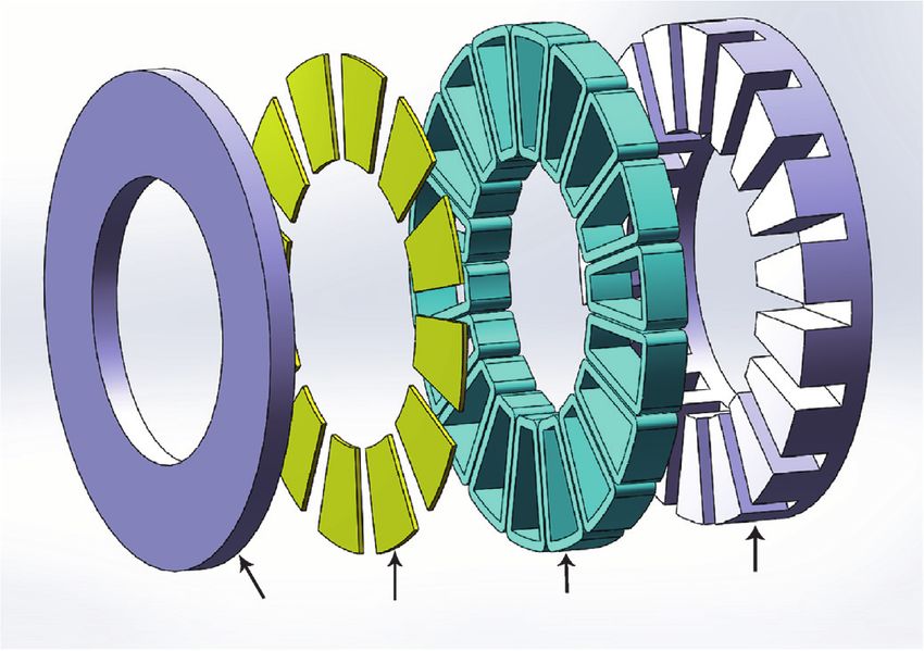
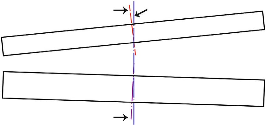
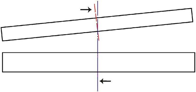
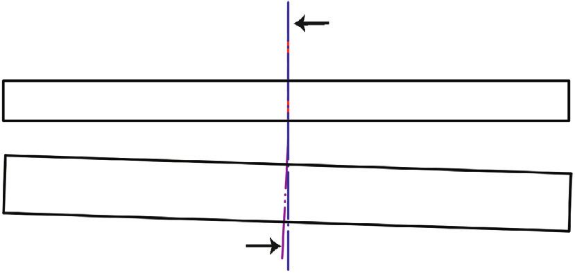
2 Mathematical Problems in Engineering

magnetic field analysis of electrical machines, some studies SC mapping is carried out with the help of the SC
equated the depth of stator slots to infinite depth in order to toolbox of MATLAB. The machine model is transformed
facilitate the calculation of mapping function [11]. However, into three planes, as shown in Figure 3. The complex var-
in practice, the ratio of slot depth to slot width is not large iables are used in the calculation of the magnetic field by the
enough to make the assumption of infinite depth slot in proposed method. In Figure 3(a), the 2D model that ob-
many AFPM machines, so the research method above will tained from the quasi-3D method is shown in the V-plane.
bring errors to the calculation of results. In Reference [12], Next, a rectangle domain in the W-plane is mapped to the
the magnetic field of an AFPM machine with slots of limited slotted air-gap polygon in the V-plane, and there is a strip
depth is analyzed by using the Schwarz–Christoffel mapping air-gap as shown in Figure 3(b). Then, a mapping is used to
method. In Reference [13], conformal transformation and map the interior of an annular domain in the T-plane to a
the EMC method are combined to study the unbalanced rectangular domain in the W-plane. The reason for choosing
force of a surface-mounted permanent magnet motor with the final transformation is that periodic boundary condition
radial flux under an eccentric state. In Reference [14], air-gap will automatically satisfy, as shown in Figure 3(c). Moreover,
flux density is calculated by using a combination of Max- Hague’s field solution in the annular air-gap is available [12].
well’s equations and the Schwarz–Christoffel mapping So, the transformation is done among these 3 planes.
method, the structure of static angular eccentricity can be The air-gap flux density BV in the V-plane is obtained as
directly drawn by the Schwarz–Christoffel mapping, and zT
 ∗
 1 1
then an analytical model is proposed to study the static BV � BT � BT � BT ,
angular eccentricity of an AFPM machine. A proper zV (zV/zT)∗ (zV/zW · zW/zT)∗
modeling method plays an important role in the process of (2)
analytical calculation in AFPM machines. In Reference [15],
the quasi-3D method is introduced, which can transform the where V, W, and T are any functions of v � υ + zi,
3D geometry of an axial flux machine to a 2D geometry. By w � x + yi, and ζ � χ + σi; zV/zW, zW/zT, zV/zT, and
modeling the investigated machine with the quasi-3D zT/zV are partial derivatives; “∗ ” represents conjugate
method, the calculation needs shorter computation time function; Bv and BT are both scalars; and BT is given in
compared with the FEM while ensuring the accuracy. Reference [12].
 On the basis of the above research, we propose a method Electromagnetic force can be obtained by integrating
for calculating the electromagnetic force of AFPM machines electromagnetic force density (EFD). In an AFPM machine,
with considerable time savings. The magnetic field of an the area that the electromagnetic force acts on is certain, so
AFPM machine under no-load condition is analyzed using the electromagnetic force directly depends on the EFD.
Schwarz–Christoffel mapping in this paper, and the Maxwell Therefore, in this paper, we directly focus on the study of
stress tensor method is used to obtain the electromagnetic EFD, in order to get the variation regularity of the elec-
force distribution of the AFPM machine, considering dif- tromagnetic force.
ferent eccentricity faults, including static, dynamic, and Applying the MST method, the axial fz and tangential ft
mixed eccentricities. The investigated AFPM machine is components of EFD are given by
shown in Figure 1, and its parameters can be found in B2z − B2t
 fz � , (3)
Table 1. The electromagnetic force acting on the stator and 2μ0
rotor is solved separately. For convenience, the following
assumptions are made: (a) the core is unsaturated and the Bz · Bt
permeability is infinite; (b) eddy current loss is neglected; ft � , (4)
 μ0
and (c) end effect is neglected.
 where Bz and Bt are the axial and tangential components of
 the air-gap flux density.
2. Magnetic Field and Electromagnetic Force
The quasi-3D method is used to model the investigated 3. Eccentricity Description
AFPM machine during the process of calculating the
magnetic field. The specific steps are shown in Figure 2. Eccentricity often occurs due to assembly and other factors
 The average radius Rk of the layer K (k � 1, 2, 3, . . ., N) in an AFPM machine, resulting in uneven air-gap of the
selected is calculated as machine. The types of eccentricity can be divided into the
 R − Ri following categories: static eccentricity (SE), dynamic ec-
 R k � Ri + o (2k − 1), (1) centricity (DE), and mixed eccentricity (ME). It is noticed
 2N
 that the stator physical axis, the rotor physical axis, and the
where Ri and Ro are the internal and external radii of the rotor rotating axis do not coincide with each other in ME, as
machine. shown in Figure 4.
 In this paper, the magnetic field at an average radius Figure 5 presents parameters required in the analysis of
(k � (N + 1) / 2) of the machine is studied; the value of k is eccentricity. In order to study the electromagnetic force in
brought into equation (1) to calculate the location of the different directions more rationally, three reference coor-
investigated layer, and the result is R � 157.75 mm. dinate systems are introduced as follows:

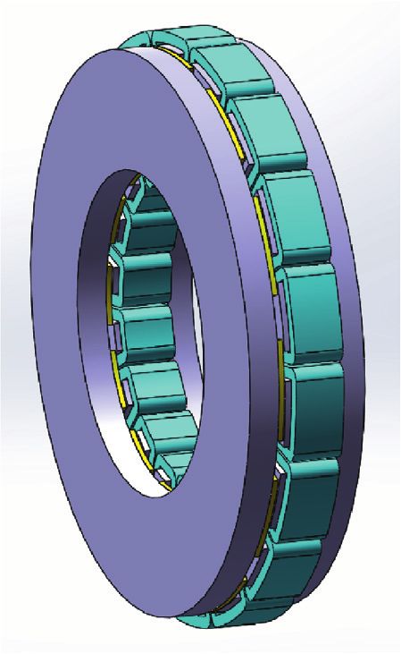
Mathematical Problems in Engineering 3

 Stator
 Rotor Magnet Winding

 (a) (b)

 Figure 1: Construction (a) and exploded view (b) of the investigated AFPM machine.

 rD
 Table 1: Parameters of the investigated machine. DEF � × 100%, (8)
 g0
Parameters Values
Rated power (kW) 1.5 where rD is the air-gap variation at the position of the
Rated speed (r/min) 150 maximum air-gap length at mean radius Rav of the rotor and
Number of stator slots 18
External radius of stator (mm) 200 rD � Rav sin βD . (9)
Internal radius of stator (mm) 115.5
Number of poles 12 The expression of air-gap length at Rav can be obtained
Axial thickness of PM (mm) 4 by introducing a time variable on the basis of equation (7),
Magnet-arc to pole-pitch ratio 0.71 and it follows that

 g(φ, t) � g0 (1 − DEF · cos(φ − c − ωt)). (10)
 (1) Machine coordinate system (MCS), based on the
 stator and rotor under ideal condition As shown in Figure 5(c), both the stator and rotor offset
 (2) Stator coordinate system (SCS), based on the stator in the case of ME. The mixed eccentricity factor (MEF) is the
 in every eccentricity fault sum of the mixed static eccentricity factor (MSEF) and the
 mixed dynamic eccentricity factor (MDEF), that is,
 (3) Rotor coordinate system (RCS), based on the rotor in
 MEF � MSEF + MDEF, and the MSEF and MDEF are as
 every eccentricity fault, and the reference is MCS
 follows:
 when the reference frame is not specified in the
 following research rMS
 MSEF � × 100%, (11)
 The eccentricity factor (EF) is introduced to describe the g0
degree of eccentricity, and the static eccentricity factor (SEF) rMD
is MDEF � × 100%, (12)
 g0
 r
 SEF � S × 100%, (5)
 g0 where rMS and rMD are the air-gap variation at the position of
where g0 is the air-gap length under ideal condition, rS is the the maximum air-gap length at Rav of the stator and rotor,
air-gap variation at the position of the maximum air-gap and they are obtained by
length at mean radius Rav of the stator, and rMS � Rav sin βMS , (13)
 rS � Rav sin βS . (6)
 rMD � Rav sin βMD . (14)
 The air-gap length under SE fault is given by Reference
[16]: And the MEF is
 g(φ) � g0 (1 − SEF · cos(φ − c)), (7) rMS + rMD
 MEF � × 100%. (15)
where φ is the angle measured from a reference point and c is g0
the reference point of minimum air-gap length. The dynamic
eccentricity factor (DEF) is obtained as The air-gap length at Rav in the case of ME is deduced as

4 Mathematical Problems in Engineering

 (a) (b) (c)

Figure 2: Modeling of an AFPM machine by the quasi-3D method. (a) N layers along the radial direction, (b) one layer taken to expand
along the circumference direction, and (c) a pair of poles of the 2D model.

 zi yi σi

 w1 w4 ζ1, ζ4
 v1 v4 χ
 ζ2, ζ3
 w2 x
 v2 v3 υ w3

 (a) (b) (c)

 Figure 3: Schwarz–Christoffel mapping. (a) V-plane, v � υ + zi; (b) W-plane, w � x + yi; and (c) T-plane, ζ � χ + σi.

 Rotor rotating axis Rotor physical axis
 (rotor physical axis)

 Rotor Rotor

 Stator Stator
 Rotor rotating axis
 Stator physical axis (stator physical axis)
 (a) (b)

 Rotor physical axis Rotor rotating axis

 Rotor

 Stator

 Stator physical axis
 (c)

 Figure 4: Eccentricity faults: (a) SE, (b) DE, and (c) ME.

g(φ,t) � g0 (1 − MDEF · cos(φ − c)) Figure 6 shows the air-gap variation of the AFPM
 machine in the case of SE, DE, and ME (SEF �30%,
 + g0 (1 − MDEF · cos(φ − c − ωt)) − g0 , DEF � 40%, and MEF � 70%, where MSEF � 30% and
 MDEF � 40%).
 � g0 1 − [MSEF · cos(φ − c) + MDEF · cos(φ − c − ωt)] .
 As can be seen from Figure 6, in the case of SE, the air-
 (16) gap length is only related to the spatial position and does not

Mathematical Problems in Engineering 5

 g0

 rD
 RCS RCS
 βD
 βS

 rS

 g0
 MCS
 MCS
 Rav
 Rav
 SCS SCS
 (a) (b)

 rMD
 RCS
 βMD

 g0
 MCS
 βMS

 Rav

 rMS
 SCS

 (c)

 Figure 5: Parameters in the analysis of eccentricity: (a) SE, (b) DE, and (c) ME.

change with time. In the case of DE and ME, the air-gap In order to describe the distortion degree of air-gap
length of a certain spatial position varies with time. When density corresponding to different EFs, the following for-
DE occurs, the maximum and minimum values of the air- mula can be obtained:
gap length at different times remain unchanged, but these THD EF2 � THD EF1 + κ EF2 − EF1 , (17)
two values vary with time in the case of ME, and the air-gap
flux density and EFD of the machine will also be affected where THD(EF2) and THD(EF1) represent the THD of air-
accordingly. gap density when the eccentricity factor is EF2 and EF1 and κ
 is the slope which is used to describe the variation degree of
 THD from THD(EF1) to THD(EF2).
3.1. Air-Gap Magnetic Field. The eccentric AFPM machine As shown in Figure 9, the κ is all positive, which indicates
model of V-plane is established in the CS. As shown in that bigger THD occurs when the EF is bigger. When the EF
Figure 7, in order to describe the change of air-gap caused by varies from 0 to 0.1, κ is rather small, and that means the air-
the eccentricity, Schwarz–Christoffel mapping described gap density is influenced less when the EF is 0.1. However,
above is used to obtain the air-gap flux density under the the value of κ increases sharply when the EF increases to 0.2.
eccentricity fault by equation (2). So, the EF should be limited to less than 0.1 for a less impact
 Because of the similarity in the calculation process of air- on air-gap density.
gap flux density in SE, DE, and ME, the DE (DEF � 40%) is
taken as an example to illustrate in detail. The calculation
results are shown in Figure 8. 3.2. Electromagnetic Force. With reference to CS, the syn-
 As shown in Figures 7 and 8, the results of flux density thetic EFD of the AFPM machine is fs, and it can be
calculated by the SC and FEM coincide with each other, and expressed as
EFD can be obtained from equations (3) and (4). That also �→ �→ �→
 f S � f z + ft . (18)
verifies the validity of the proposed method in calculating
electromagnetic force. In the following analysis, EFD is decomposed into axial
 From the combination of Figures 7 and 8, it can be seen and tangential components in different reference coordinate
that the axial air-gap flux density has changed significantly systems (SCS, MCS, and RCS). The analysis process for each
under eccentric condition, and the tangential component is of the three kinds of eccentricity is very similar to any of
influenced, but to a lesser extent. In the range of 0–90 them, so only the transformation for ME is given in this
degrees, the axial component is smaller than that of the ideal paper, and the analysis for SE and DE can be easily done with
condition, and the reduced value decreases with the increase the help of Figures 10(a) and 10(b).
of the mechanical angle. For ME, the reference is RCS, when the force acting on
 In the range of 90–180 degrees, the air-gap length of the the rotor is analyzed. And when analyzing the force acting
eccentricity state is less than that of the normal state, so the on the stator, the reference is SCS. Referring to
axial component of the air-gap flux density is larger than that Figure 10(c), the expression of EFD in ME can be obtained.
of the normal state, and the increased value increases with ′ and fMst
 fMsz ′ are the axial and tangential components of
the increase of the mechanical angle. the EFD acting on the stator, and f′Mrz and f′Mrt are those

6 Mathematical Problems in Engineering

 1.4 1.4

 1.3 1.3

 1.2 1.2
 Air-gap length (mm)

 Air-gap length (mm)
 1.1 1.1

 1 1

 0.9 0.9

 0.8 0.8

 0.7 0.7

 0.6 0.6
 0 60 120 180 240 300 360 0 60 120 180 240 300 360
 Angular position (mechanical degree) Angular position (mechanical degree)
 t1 t1
 t2 t2

 (a) (b)
 1.4

 1.3

 1.2
 Air-gap length (mm)

 1.1

 1

 0.9

 0.8

 0.7

 0.6
 0 60 120 180 240 300 360
 Angular position (mechanical degree)
 t1
 t2

 (c)

 Figure 6: Air-gap variation of the AFPM machine: (a) SE, (b) DE, and (c) ME.

acting on the rotor. Then, the following expressions are eccentricity fault, and the degree of the influence is related to
easily obtained: the EF.
 In Figures 11–19, the angular positions of the minimum
 ′ � fs · sin βMS + ξ MS ,
 fMsz air-gap length gmin and the maximum air-gap length gmax
 ′
 fMst � fs · cos βMS + ξ MS , are as follows:
 (19)
 ′ � fs · cos βMD + ξ MD ,
 fMrz SE: gmin � 0.7 mm, mechanical degree: 0;
 f′Mrt � fs · sin βMD + ξ MD , gmax � 1.3 mm, mechanical degree: 180
 DE: gmin � 0.6 mm, mechanical degree: 180;
where ξ MS � ⟨fs , ft ⟩ and ξ MD � ⟨fs , fz ⟩. gmax � 1.4 mm, mechanical degree: 0
 ME: gmin � 0.3 mm, mechanical degree: 0;
4. Results and Discussion gmax � 1.7 mm, mechanical degree: 180

The EFD acting on the stator and rotor under different From Figures 11–20, the followings conclusions can be
eccentricity faults can be depicted in Figures 11–19. drawn:
 From the comparison among Figures 11–20, it can be (1) As shown in Figures 11, 12, 14, 15, 17, and 18, the
seen that EFD of the AFPM machine is affected in any EFD increases at the position where the air-gap

Mathematical Problems in Engineering 7

 Eccentric condition Healthy condition

 Figure 7: Eccentric AFPM machine model of the V-plane.

 1.5
 0.6

 1.0 0.4

 0.5

 Flux density (T)
 0.2
 Flux density (T)

 0.0 0.0

 –0.5 –0.2

 –1.0 –0.4

 –1.5 –0.6
 0 30 60 90 120 150 180 0 30 60 90 120 150 180
 Angular position (mechanical degree) Angular position (mechanical degree)

 SC (healthy condition) SC (DE) SC (healthy condition) SC (DE)
 FEM (healthy condition) FEM (DE) FEM (healthy condition) FEM (DE)
 (a) (b)

 Figure 8: Axial (a) and tangential (b) components of the air-gap flux density in DE (DEF � 40%).

 1.4
 1.2
 1.0

 κ 0.8
 0.6
 0.4
 0.2
 0.0
 0.1_0

 0.2_0.1

 0.3_0.2

 0.4_0.3

 0.5_0.4

 0.6_0.5

 0.7_0.6

 0.8_0.7

 0.9_0.8

 EF2_EF1

 Figure 9: Variation of κ with different EFs.

 length decreases due to eccentricity and decreases at square of the axial and tangential flux density
 the position where the air-gap length increases. By according to equation (3), and the tangential EFD is
 comparing the (a) and (b) of Figures 11, 12, 14, 15, in direct proportion to the product of axial and
 17, and 18 with Figure 20, it can be seen that ec- tangential flux density on the basis of equation (4).
 centricities have a greater impact on axial compo- Moreover, the results obtained from Figure 8 show
 nents of EFD rather than tangential components. that the axial flux density is much larger than the
 And that can also be judged from the (c) of Fig- tangential in most locations. As a result, the axial
 ures 11, 12, 14, 15, 17, and 18. The main reason is that component of EFD suffers a greater impact brought
 the axial EFD is proportional to the difference of the by eccentricity.

8 Mathematical Problems in Engineering

 f ′Ssz fz = fDsz fs
 fz = fSrz fs RCS f′Drz
 RCS βD
 MCS βD ξD
 βS MCS f′Drt
 SCS
 ξS ft = fDst
 SCS ft = fSrt
 βS f ′Sst
 (a) (b)
 f′Msz
 fz fs
 RCS
 f ′Mrz
 βMD
 MCS
 βMD ξMD
 βMS
 ξMS f Mrt
 ′
 SCS
 ft
 βMS f′Mst

 (c)

 Figure 10: Decomposition of EFD: (a) SE, (b) DE, and (c) ME.

 600 90 600 90
 120 60 120 60
 400 400
 150 30 150 30
 200 200
 EFD (kpa)

 EFD (kpa)

 0 180 0 0 180 0

 200 200
 210 330 210 330
 400 400

 600 240 300 600 240 300
 270 270
 Axial component Tangential component
 (a) (b)

 80
 60
 40
 20
 EFD (kpa)

 0
 –20
 –40
 –60
 –80
 0 60 120 180 240 300 360
 Angular position (mechanical degree)
 Axial component
 Tangential component
 (c)

Figure 11: SE: EFD at different positions of the stator at R � 157.75 mm (SEF � 0.3), including axial (a) and tangential (b) components and
(c) axial and tangential components of the difference with ideal condition.

Mathematical Problems in Engineering 9

 600 90 600 90
 120 60 120 60
 400 400
 150 30 150 30
 200 200
 EFD (kpa)

 EFD (kpa)
 0 180 0 0 180 0

 200 200
 210 330 210 330
 400 400

 600 240 300 600 240 300
 270 270
 Axial component Tangential component
 (a) (b)

 80
 60
 40
 20
 EFD (kpa)

 0
 –20
 –40
 –60
 –80
 0 60 120 180 240 300 360
 Angular position (mechanical degree)
 Axial component
 Tangential component
 (c)

Figure 12: SE: EFD at different positions of the rotor at R � 157.75 mm (SEF � 0.3), including axial (a) and tangential (b) components and (c)
axial and tangential components of the difference with ideal condition.

 1.2

 0.8

 0.4
 EFD (kpa)

 0.0

 –0.4

 –0.8

 –1.2

 0 60 120 180 240 300 360
 Angular position (mechanical degree)
 Axial component
 Tangential component
 Figure 13: SE: Difference of EFD at different positions between the stator and rotor at R � 157.75 mm (SEF � 0.3).

10 Mathematical Problems in Engineering

 600 90 600 90
 120 60 120 60
 400 400
 150 30 150 30
 200 200
 EFD (kpa)

 EFD (kpa)
 0 180 0 0 180 0

 200 200
 210 330 210 330
 400 400

 600 240 300 600 240 300
 270 270
 Axial component Tangential component
 (a) (b)

 40

 20
 EFD (kpa)

 0

 –20

 –40

 0 60 120 180 240 300 360
 Angular position (mechanical degree)
 Axial component
 Tangential component
 (c)

Figure 14: DE: EFD at different positions of the stator at R � 157.75 mm (DEF � 0.4), including axial (a) and tangential (b) components and
(c) axial and tangential components of the difference with ideal condition.

 (2) In the corresponding coordinate system, the axial In addition, there are still some issues about the EFD
 force acting on the stator is larger than that acting on worth discussing. Taking DE as an example as before, the
 the rotor, and the tangential force acting on the following research is done.
 stator is smaller. The results are consistent with the As shown in Figure 21, EFD varies linearly with radius.
 analysis in Figure 10. Therefore, attention should be On the air-gap reduction side, outer position's EFD is larger
 paid to the axial force acting on the stator when than the inner one’s because of the gradual reduction of air-
 eccentricity occurs. In practical application, a thrust gap length, while it does the opposite on the air-gap en-
 bearing with supporting axial load capacity can be largement side.
 installed in the stator. When solving the EFD under eccentric conditions
 (3) The EFs in the three kinds of eccentricity are dif- within one electrical period, the proposed analytical method
 ferent: SEF � 0.3, DEF � 0.4, and MEF � 0.7. Among takes 2 minutes to calculate, while the 3D FEM takes 12
 the three eccentricities, the variation of the EFD hours to complete the calculation. So, the computation time
 under ME is the largest because of its largest EF. The of the proposed analytical method is much less than that of
 larger the EF, the larger the air-gap length changes. the FEM. The proposed analytical method can be a useful
 So, the air-gap density and the EFD will be more tool for analyzing AFPM machines.
 affected. So, if eccentricity faults cannot be avoided When eccentricity occurs, the air-gap field is dis-
 in practical use, measures such as improving as- torted, which makes the axial EFD distorted compared
 sembly accuracy should be taken to weaken the with that of ideal condition. The spatial decomposition of
 degree of eccentricity. axial EFD is done under both ideal and eccentricity

Mathematical Problems in Engineering 11

 600 90 600 90
 120 60 120 60
 400 400
 150 30 150 30
 200 200
 EFD (kpa)

 EFD (kpa)
 0 180 0 0 180 0

 200 200
 210 330 210 330
 400 400

 600 240 300 600 240 300
 270 270
 Axial component Tangential component
 (a) (b)

 40

 20
 EFD (kpa)

 0

 –20

 –40

 0 60 120 180 240 300 360
 Angular position (mechanical degree)
 Axial component
 Tangential component
 (c)

Figure 15: DE: EFD at different positions of the rotor at R � 157.75 mm (DEF � 0.4), including axial (a) and tangential (b) components and
(c) axial and tangential components of the difference with ideal condition.

 1.2

 0.8

 0.4
 EFD (kpa)

 0.0

 –0.4

 –0.8

 –1.2

 0 60 120 180 240 300 360
 Angular position (mechanical degree)
 Axial component
 Tangential component
Figure 16: DE: Axial and tangential components of the difference of EFD at different positions between the stator and rotor at
R � 157.75 mm (DEF � 0.4).

12 Mathematical Problems in Engineering

 600 90 600 90
 120 60 120 60
 400 400
 150 30 150 30
 200 200
 EFD (kpa)

 EFD (kpa)
 0 180 0 0 180 0

 200 200
 210 330 210 330
 400 400

 600 240 300 600 240 300
 270 270
 Axial component Tangential component
 (a) (b)

 120

 80

 40
 EFD (kpa)

 0

 –40

 –80

 0 60 120 180 240 300 360
 Angular position (mechanical degree)
 Axial component
 Tangential component
 (c)

Figure 17: ME: EFD at different positions of the stator at R � 157.75 mm (MEF � 0.7), including axial (a) and tangential (b) components and
(c) axial and tangential components of the difference with ideal condition.

conditions, and the main spatial order is given in Fig- performance of the machine in an all-round way. In order to
ure 22. On the basis of the original spatial order, the ± 1 avoid excessive shunting of the permanent magnet flux, the
and ± 2 components appear because of the eccentricity. machine with semiclosed slots under eccentricity condition
And the EFD magnitude of the ± 2 order is relatively is investigated.
small. Some of the extra spatial orders of axial EFD will be The spatial order of EFD of the original model
closer to the lower orders of the stator, which will ag- (Figure 23(a).) and the model with a magnetic wedge
gravate the vibration of the motor. The change of EFD (Figure 23(b)) is illustrated in Table 2. In Table 2, it is shown
caused by eccentricity will affect the vibration and noise that all the spatial harmonics except the 12th order are
characteristics of the motor. smaller when the stator slots are semiclosed. Especially, the
 Open slot structures are more favorable for original sixth harmonic with a smaller order and larger
manufacturing. As shown in Figure 22, the large harmonic amplitude has been weakened obviously. Therefore, when
amplitude of axial EFD will aggravate the vibration of the eccentricity occurs, vibration of the AFPM with semiclosed
motor. In motor design, it has been demonstrated in Ref- slots will be significantly lower than that of the AFPM with
erences [17] and [18] that magnetic wedges can improve open slots.

Mathematical Problems in Engineering 13

 600 90 600 90
 120 60 120 60
 400 400
 150 30 150 30
 200 200
 EFD (kpa)

 EFD (kpa)
 0 180 0 0 180 0

 200 200
 210 330 210 330
 400 400

 600 240 300 600 240 300
 270 270
 Axial component Tangential component
 (a) (b)

 120

 80

 40
 EFD (kpa)

 0

 –40

 –80

 0 60 120 180 240 300 360
 Angular position (mechanical degree)
 Axial component
 Tangential component
 (c)

Figure 18: ME: EFD at different positions of the rotor at R � 157.75 mm (MEF � 0.7), including axial (a) and tangential (b) components and
(c) axial and tangential components of the difference with ideal condition.

 2

 1
 EFD (kpa)

 0

 –1

 –2

 –3
 0 60 120 180 240 300 360
 Angular position (mechanical degree)
 Axial component
 Tangential component
Figure 19: ME: Axial and tangential components of the difference of EFD at different positions between the stator and rotor at
R � 157.75 mm (MEF � 0.7).

14 Mathematical Problems in Engineering

 600 90 600 90
 120 60 120 60
 400 400
 150 30 150 30
 200 200
 EFD (kpa)

 EFD (kpa)
 0 180 0 0 180 0

 200 200
 210 330 210 330
 400 400

 600 240 300 600 240 300
 270 270
 Axial component Tangential component
 (a) (b)

 Figure 20: Axial and tangential components of the EFD at R � 157.75 mm under ideal condition.

 400

 350
 EFD (kpa)

 300

 250
 120 140 160 180 200
 R (mm)
 Air-gap reduction side
 Air-gap enlargement side
 Figure 21: EFD at different radii.

 200 200

 150 150
 EFD (kpa)

 EFD (kpa)

 100 100

 50 50

 0 0
 0 6 12 18 0 3 6 9 12 15 18
 Spatial order Spatial order
 (a) (b)

 Figure 22: Spatial decomposition of EFD: (a) ideal condition and (b) eccentricity condition.

Mathematical Problems in Engineering 15

 Magnetic wedge

 (a) (b)

 Figure 23: Open slot (a) and semiclosed slot (b) 2D models.

 Table 2: Spatial orders of EFD of the open slot and the semiclosed slot AFPM machine.
Spatial order 1 2 4 5 6 7
Open slot 33 3.07 0.62 6.21 53.3 4.6
Semiclosed slot 32.3 0.46 0.59 0.27 5.12 0.5
Spatial order 8 10 11 12 13 14
Open slot 0.93 0.73 12.7 133.1 12.3 0.6
Semiclosed slot 0.75 0.49 11.87 144.4 11.8 0.4
Spatial order 16 17 18 19 20
Open slot 1.7 16.4 103.5 8.3 0.9
Semiclosed slot 0.9 1.4 10.8 0.8 0.6

5. Conclusions [2] D. K. Lim, Y. S. Cho, J. S. Ro, S. Y. Jung, and H. K. Jung,
 “Optimal design of an axial flux permanent magnet syn-
This paper introduced a fast analytical method to study the chronous motor for the electric bicycle,” IEEE Transactions on
electromagnetic force of eccentric AFPM machines, and the Magnetics, vol. 52, no. 3, 2016.
results are verified by the FEM. The analytical method is [3] C. Kim, G. Jang, J. Kim, J. Ahn, C. Baek, and J. Choi,
based on the Schwarz–Christoffel mapping and MST “Comparison of axial flux permanent magnet synchronous
 machines with electrical steel core and soft magnetic composite
method. The expression of air-gap length in ME is obtained.
 core,” IEEE Transactions on Magnetics, vol. 53, no. 11, 2017.
EFD is used to characterize the variation of electromagnetic [4] W. Deng and S. Zuo, “Axial force and vibroacoustic analysis of
force. EFD is decomposed into axial and tangential com- external-rotor axial-flux motors,” IEEE Transactions on In-
ponents in different reference coordinate systems (SCS, dustrial Electronics, vol. 65, no. 3, pp. 2018–2030, 2018.
MCS, and RCS) during the analysis of electromagnetic force [5] L. Zeng, X. Chen, W. Li, X. Jiang, and X. Luo, “A thrust force
acting on the stator and rotor. The method can be used in analysis method for permanent magnet linear motor using
different eccentricities, including SE, DE, and ME. The Schwarz-Christoffel mapping and considering slotting effect,
distribution law of electromagnetic force under different end effect, and magnet shape,” IEEE Transactions on Mag-
eccentricity conditions is summarized to facilitate further netics, vol. 51, no. 9, pp. 1–9, 2015.
research on motor design, eccentricity detection, and so on. [6] A. D. Gerlando, G. M. Foglia, M. F. Iacchetti, and R. Perini,
The method presented in this paper has a strong universality “Evaluation of manufacturing dissymmetry effects in axial flux
 permanent-magnet machines: analysis method based on field
and is applicable to AFPM machines under both eccentric
 functions,” IEEE Transactions on Magnetics, vol. 48, no. 6,
and ideal conditions. pp. 1995–2008, 2012.
 [7] B. M. Ebrahimi, J. Faiz, and M. J. Roshtkhari, “Static-, dy-
Data Availability namic-, and mixed-eccentricity fault diagnoses in permanent-
 magnet synchronous motors,” IEEE Transactions on Indus-
All data included in this study are available upon request to trial Electronics, vol. 56, no. 11, pp. 4727–4739, 2009.
the corresponding author. [8] M. Aydin and M. Gulec, “A new coreless axial flux interior
 permanent magnet synchronous motor with sinusoidal rotor
 segments,” IEEE Transactions on Magnetics, vol. 52, no. 7,
Conflicts of Interest p. 8105204, 2016.
 [9] D. Kim, M. Noh, and Y. W. Park, “Unbalanced magnetic
The authors declare no conflicts of interest. forces due to rotor eccentricity in a toroidally-wound BLDC
 motor,” IEEE Transactions on Magnetics, vol. 52, no. 7,
References p. 8203204, 2016.
 [10] T. A. Driscoll and L. N. Trefethen, Cambridge Monographs on
 [1] M. Aydin, S. Surong Huang, and T. A. Lipo, “Torque quality Applied and Computational Mathematics, Cambridge Uni-
 and comparison of internal and external rotor axial flux versity Press, Cambridge, U.K, 2002.
 surface-magnet disc machines,” IEEE Transactions on In- [11] X. H. Wang, Q. F. Li, S. H. Wang, and Q. F. Li, “Analytical
 dustrial Electronics, vol. 53, no. 3, pp. 822–830, 2006. calculation of air-gap magnetic field distribution and

16 Mathematical Problems in Engineering

 instantaneous characteristics of brushless DC motors,” IEEE
 Transactions on Energy Conversion, vol. 18, no. 3, pp. 424–432,
 2003.
[12] A. Alipour and M. Moallem, “Analytical magnetic field
 analysis of axial flux permanent-magnet machines using
 Schwarz-Christoffel transformation,” in Proceedings of the
 2013 International Electric Machines & Drives Conference,
 pp. 670–677, Chicago, IL, USA, May 2013.
[13] F. Rezaee-Alam, B. Rezaeealam, and J. Faiz, “Unbalanced
 magnetic force analysis in eccentric surface permanent-
 magnet motors using an improved conformal mapping
 method,” IEEE Transactions on Energy Conversion, vol. 32,
 no. 1, pp. 146–154, 2017.
[14] B. Guo, Y. Huang, and F. Peng, “An improved conformal
 mapping method for static angular eccentricity analysis of
 axial flux permanent magnet machines,” Journal of Magnetics,
 vol. 23, no. 1, pp. 27–34, 2018.
[15] A. Parviainen, M. Niemela, and J. Pyrhonen, “Modeling of
 axial flux permanent-magnet machines,” IEEE Transactions
 on Industry Applications, vol. 40, no. 5, pp. 1333–1340, 2004.
[16] S. M. Mirimani, A. Vahedi, F. Marignetti, and R. Di Stefano,
 “An online method for static eccentricity fault detection in
 axial flux machines,” IEEE Transactions on Industrial Elec-
 tronics, vol. 62, no. 3, pp. 1931–1942, 2015.
[17] G. D. Donato, F. G. Capponi, and F. Caricchi, “Influence of
 magnetic wedges on the no-load performance of axial-flux
 permanent-magnet machines,” Proceedings of 2010 IEEE In-
 ternational Symposium on Industrial Electronics, vol. 27,
 pp. 1333–1339, 2010.
[18] G. D. Donato, F. G. Capponi, and F. Caricchi, “Influence of
 magnetic wedges on the load performance of axial-flux per-
 manent-magnet machines,” Proceedings of 36th Annual
 Conference on IEEE Industrial Electronics Society, vol. 24,
 pp. 876–882, 2010.