Magnetic particle imaging using linear magnetization response-driven harmonic signal of magnetoresistive sensor
←
→
Page content transcription
If your browser does not render page correctly, please read the page content below
Applied Physics Express

LETTER • OPEN ACCESS

Magnetic particle imaging using linear magnetization response-driven
harmonic signal of magnetoresistive sensor
To cite this article: Suko Bagus Trisnanto et al 2021 Appl. Phys. Express 14 095001

View the article online for updates and enhancements.

                               This content was downloaded from IP address 46.4.80.155 on 22/09/2021 at 02:47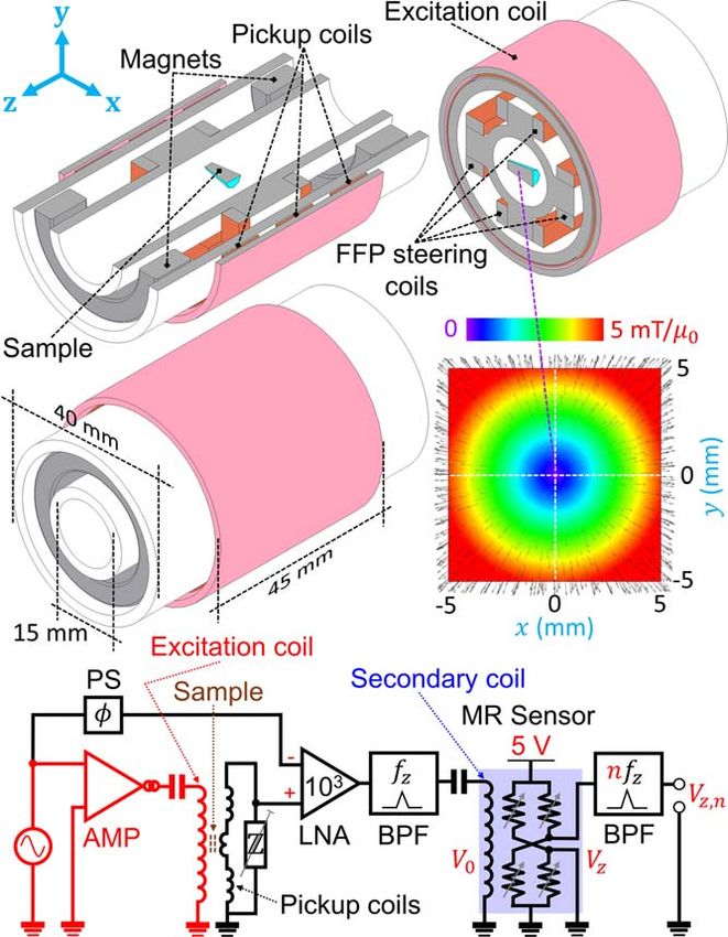
Applied Physics Express 14, 095001 (2021)                                                                                                   LETTER
https://doi.org/10.35848/1882-0786/ac1d63

Magnetic particle imaging using linear magnetization response-driven harmonic
signal of magnetoresistive sensor
Suko Bagus Trisnanto1* , Tamon Kasajima2, Taiju Akushichi2, and Yasushi Takemura1*
1
    Department of Electrical and Computer Engineering, Yokohama National University, Yokohama 240-8501, Japan
2
    Technology and Intellectual Property HQ, TDK Corporation, Tokyo 103-6128, Japan
*
E-mail: suko-trisnanto-zt@ynu.ac.jp; takemura-yasushi-nx@ynu.ac.jp
Received June 3, 2021; revised July 27, 2021; accepted August 12, 2021; published online August 27, 2021

     We achieved a harmonic-rich signal from linear magnetization responses of magnetic nanoparticles under 40 μT/μ0 excitation field to facilitate
     magnetic particle imaging (MPI). In contrast, large harmonic responses are typically attributed to the nonlinear field-dependent magnetization
     characteristics of the particles, thus questioning technical and clinical issues toward a human-sized MPI scanner. By using a magnetoresistive
     sensor, we propose a strategy to exploit the linear responses of the tracers at low field regime where the standard MPI may struggle with spatial
     signal decoding. The achieved high-contrast images of a solid ferucarbotran phantom bring new expectation toward clinical use of MPI.
     © 2021 The Japan Society of Applied Physics

M
          agnetic particle imaging (MPI) is a tomographic                      excitation frequency requires careful signal processing to
          imaging method which utilizes magnetic nanoparti-                    anticipate the feedthrough contamination of the fundamental
          cles as tracers for tracking stem cells, locating and                frequency.13) Hence, the harmonic responses of MR sensor
heating tumors, visualizing organ perfusion and blood                          may facilitate the MPI scanner for human torso to be cost-
pooling, as well as for biomedical research applications.1–5)                  and time-efficient.
MPI works as a noninvasive technique by inducing ac                               Regarding how an MR sensor is applicable for MPI
magnetic field to the tracers under a static field gradient,                     system, Fig. 1 highlights a transformation from a single-
thus the acquired tracer-sensitive signal is spatially                         frequency magnetic signal of the tracers into a harmonic-rich
dependent.6) The superparamagnetism of magnetic nanopar-                       signal of the sensor. In principle, magnetic nanoparticles
ticles become a main contributor of this feature in which the                  shows virtually no harmonic magnetization spectra induced
dynamically magnetized particles exhibit harmonic compo-                       by small ac field within the linear response regime.14) Thus,
nents of magnetization response under a large ac field;                         for this situation, only the magnetic response at fundamental
however, the dc field further reduces the harmonic                              frequency remains spatially field-dependent and attributable
magnitudes.7) Therefore, by introducing a field-free region                     to tracer distribution (Fig. 1).13) The MR sensor can detect
(e.g. point and line) within the field gradient and scanning it                 this monotone signal proportionally as a field to saturate the
across the tracers, MPI should achieve a high signal-to-noise                  sensor output. The resulting harmonic signals are adjustable
ratio (SNR) of the harmonic signals to locate and image the                    to satisfy high SNR for further MPI signal processing. The
tracers in real-time.8) Recently, MPI can even identify                        MR sensor also offers low noise density and flexible dynamic
cellular uptake of magnetic nanoparticles in the order of                      range of the harmonics, in addition to simple circuital design.
0.1 ng iron mass concentration per cell.5)                                     In this letter, we demonstrate the implementation of MR
   Since the standard MPI is strictly dependent on the                         sensor in MPI system by emphasizing the harmonic signal
nonlinear field-dependent magnetization properties of the                       characteristics and the optimization of image reconstruction.
tracers, it bears technical problems in realizing a human-                        We build a miniaturized MPI scanner with 15 mm bore
sized MPI scanner.9) In addition to the magnetostimulation                     size, which is equipped with 2 ring magnets to create the
limits on human body,10) the issue is related to the inefficient                FFP, as shown in Fig. 2. The measured field gradient along z
ac field generation at high frequency (e.g. typically around                    axis is 1.6 T m−1, whereas magnetic field simulation by
25 kHz) and field amplitude (e.g. above 5 mT/μ0), as well as                    JMAG Designer 19.0 (JSOL Corp., Japan) confirms
creating the field gradient (e.g. around 2 T m−1). Even though                  0.8 T m−1 on both x and y axes. The scanner adopts our
the gradient can be set to 0.2 T m−1 for a human brain MPI                     previous MPI scenario while recording the magnetization
scanner,11) reducing the field amplitude remains a challenge                    response of the tracers at z axis by a gradiometric receive
as it leads to the linear magnetization response of the tracers                coil.13) Figure 2 further describes the instrumentation setup of
with no observable harmonics. Here, we propose a method to                     the sensing system in which consists of a 10 kHz excitation
transform a monotone magnetic signal into harmonic-rich                        coil connected to a function generator-driven power amplifier
signal by utilizing saturation properties of a magnetoresistive                (i.e. Picotest G5100A and NF Corp. HSA 4011). The driving
(MR) sensor. This technique is designed to operate an MPI                      field amplitude is set at 40 μT/μ0; μ0 is magnetic permeability
scanner under extremely low oscillatory excitation field                        of free space. The detected electromotive force from the
below the geomagnetism. Meanwhile, we previously intro-                        receive coil is then amplified 1000-folds along with a
duce a modulated MPI implementing high-frequency excita-                       compensation voltage from phase shifter, prior to filtering
tion field to encode linear Neél relaxation response with a                     at 10 kHz band-pass. Here, we later define the resulting
time-varying field-free point (FFP) coordinate.12) However,                     voltage as V0.
the resulting MPI signal at narrow sidebands around the

                Content from this work may be used under the terms of the Creative Commons Attribution 4.0 license. Any further distribution of this
                work must maintain attribution to the author(s) and the title of the work, journal citation and DOI.

                                                                       095001-1                        © 2021 The Japan Society of Applied Physics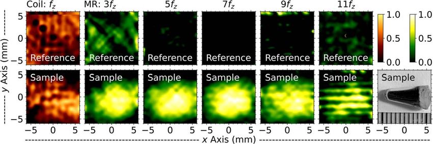
Appl. Phys. Express 14, 095001 (2021) S. B. Trisnanto et al.
Fig. 1. (Color online) Signal characterization pathway of MPI with MR
sensor. An extremely low ac magnetic field is used to drive linear
magnetization response of magnetic nanoparticles (M/MS). Monotone mag-
netic signal (dM/dt) at fundamental frequency f1 is then transformed by the
MR sensor into harmonic components with fn = nf1 for n = 2, 3, 4... due to
its nonlinear properties. The particle response for a spatially different dc field
(e.g. red and black lines) can be identified from the change in harmonic
components of the sensor output.
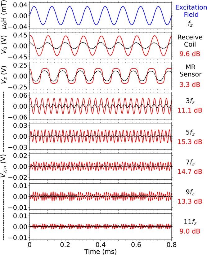
Fig. 3. (Color online) Harmonic signal decomposition of MR sensor
output. A 40 μT/μ0 sinusoidal magnetic field at fz = 10 kHz applied to a
4 mg solid Resovist® sample results in linear magnetic response in terms of
V0 as detected by the receive coil. Proportional to the field from the
secondary coil, the MR sensor output (Vz) saturates and leads to odd
harmonic components (Vz,n) with high signal integrity for n ⩽ 7; however,
even harmonic components are neglected. The red solid lines and black
dashed lines represent signals from the sample and sample-free reference,
respectively.
To provide a harmonic-rich signal proportional to the
magnetic response of the tracers, we directly couple V0 to a
secondary coil near the MR sensor (i.e. TDK Corp. Nivio
xMR sensor) to enable flux transformer circuit. Nivio xMR
sensor has remarkable sensitivity to benefit
magnetocardiography.15) While placing the sensor far from
the MPI scanner, we set dc bias to cancel the geomagnetic
field which initially saturates the sensor output. As shown in
Fig. 2, the MR sensor is powered by 5 V dc voltage and
connected to the programmable band-pass filter (i.e. NF
Corp. 3627), thus the MR sensor output voltage (Vz) can be
tuned to harmonic signal Vz,n with frequency of nfz. We
intentionally adjust V0 (e.g. via controlling the output of
phase shifter) so that the nth harmonic order of the z axis
excitation frequency fz = 10 kHz is up to n = 11. In this case,
Fig. 2. (Color online) Design of MPI scanner connected to ex situ MR Fig. 3 shows a preliminary result of the signal characteristics
sensor circuit. Two ring magnets are oppositely installed to create FFP with of the MR sensor. Expressing SNR as a logarithmic ratio of
0.8 T m−1 on the x and y axes, and 1.6 T m−1 on the z axis, as simulated by signal power (e.g., maximum V02 , Vz2 , and Vz2, n ) to the
JMAG Designer 19.0. The z-axis magnetic signal is measured by a
gradiometric receive coil (i.e. a combination of 3 pickup coils), 1000-fold
reference (at the same impedance), MR sensor output appears
amplified, and filtered at frequency fz as V0, prior to driving secondary coil to have better SNR of low-order harmonic components than
near the MR sensor. Vz,n, harmonic signal of Vz, is selectively recorded for the receive coil.
the image reconstruction. AMP, PS, LNA, and BPF stand for power At the fundamental frequency, the magnetic signal from
amplifier, phase shifter, low noise amplifier, and band-pass filter, respec- the tracers mixes with that from the excitation field, thus
tively.
requiring a signal separation.16,17) From Fig. 3, the amplitude
increment of V0 indicates magnetization response of the
tracers. Here, a solid ferucarbotran (Fujifilm RI Pharma,
095001-2 © 2021 The Japan Society of Applied Physics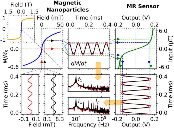
Appl. Phys. Express 14, 095001 (2021) S. B. Trisnanto et al.
Japan) sample was placed inside the scanner without moving where Mx and My are magnetization components induced by
the FFP relatively. The unbalanced gradiometric receive coil FFP steering fields Hx = Hx ˆix and Hy = Hy ˆiy , and Mz is the
can lead to a non-zero V0 when detecting no sample (e.g. response for the excitation field Hz = Hz ˆiz .13) Here, ˆix , ˆiy ,
black lines attributed to sample-free reference voltage) at and ˆiz are axial unit vectors for x, y, and z axes. From Eq. (1),
40 μT/μ0 ac field. We apply an additional signal tuned by the relaxation modulation occurs with ax and ay as the
phase shifter as a correction voltage which is further fed to a amplitude sensitivities for Mx(t) and My(t), respectively.
differential amplifier (i.e. NF Corp. 5307) together with the The signal amplification K includes the geometric sensitivity
output voltage from the receive coil. To obtain tracer- of the receive coil and the gain from low noise amplifier
sensitive 11th harmonic signal, the reference voltage is (Fig. 2). Since V0 connected to an inductor (i.e. secondary
necessarily increased. Figure 3 identifies severe distortion of coil near MR sensor) with inductance L, the resulting
Vz,n above 9fz which potentially affects the image reconstruc- i0(t) = ∫[V0(t)/L]dt can be further expressed by Eq. (2) as
tion. Harmonic decomposition of Vz into Vz,n is meaningful - m 0 Kn
for the odd components since the nonlinear characteristics of i 0 (t ) = [1 + ax Mx (t ) + a y My (t )] Mz (t ) , (2 )
L
MR sensor resemble Langevin function.18) However, Vz,n
with low signal integrity and small magnitude for n = 2, 4, 6, which creates magnetic field H0 to be detected by the MR
… is inconvenient for the modulated MPI. sensor. For a given 5 V power supply, the sensor output Vz(t)
Unlike V0 (i.e. electromotive force of pickup coil), Vz may saturate depending on i0(t) ∝ H0(t) as
differs 180° relative to the excitation field. Flux transformer Vz = Vz , s (H0) , (3 )
circuit (Fig. 2) inverts the signal while the MR sensor detects
the field from inductive current i0 flowing through the where Vz,s = 208 mV is the saturation voltage and the field
secondary coil; phase difference between i0 and V0 is 90°. dependence of the sensor output, (H0 ), appears identical to
Depending on particle size and FFP steering frequencies ( fx the phenomenological paramagnetic Langevin function.
and fy), relaxation effects may also result in phase delay of From Eq. (3), we extract Vz,n(t), the nth harmonic
Vz(t) relative to the time-varying FFP movement on x and y component of Vz(t), for n = 3, 5, 7, 9, and 11. We implement
axes, x(t) and y(t).19) Although MPI relies on the magnitude a synchronous envelope tracking to demodulate Vz,n(t) into
of the harmonic signals, phase difference potentially affects dVz,n(t), which is followed by direct mapping of dVz,n(t) at
time-domain image reconstruction.20) We then adopt time full-width-half-maximum against the time-varying FFP co-
shifting Δt to correct signal mismatch between Vz(t + Δt), x ordinate for x(t) = Hx(t)/Gx and y(t) = Hy(t)/Gy at an equidi-
(t), and y(t).13) This phase correction is also required to stant time interval tn = (nfz )-1. The field gradient on the x and
compensate the instrumentation delay. In this letter, we y axes, Gx = Gy, are symmetric, as shown in Fig. 2, and
demonstrate MR sensor as part of magnetic sensing unit for satisfies Maxwell’s equation.21) From Fig. 4, we confirm that
the modulated MPI scanner. We used a cone-shaped solid the spatially decoded signal dVz,n(x, y) can reconstruct two-
phantom made of ferucarbotran with 4 mg iron oxide mass. dimensional image of the phantom. In comparison with
The phantom was imaged at fx = 500 Hz, fy = 501.25 Hz, and dV0(x, y) plot of the receive coil, we obtained high image
fz = 10 kHz for 0.4 s record length of all signals and 40 μT/μ0 contrast of dVz,n(x, y) relative to each artifact (i.e. sample-free
excitation amplitude. reference image). Figure 4 also indicates that n = 5 is an
When applying Hx⊥Hy⊥Hz fields to the sample with optimum order of harmonic components to replicate phantom
volume ν, the signal detected by the receive coil, V0, equals geometry. Nevertheless, changing V0 dynamic range or using
different combination of coils and MR sensor may shift the
{
V0 (t ) = - m 0 Kn [1 + ax Mx (t ) + a y My (t )]
dMz (t )
dt
frequency of the optimum harmonic signal. Image quality
appears to correlate with the characteristics of each harmonic
dMx (t ) dMy (t ) ⎤ signal Vz,n (Fig. 3).22) Here, we basically performed re-
+ ⎡ax + ay Mz (t )⎫ , (1 )
⎣ dt dt ⎦ ⎬
⎭ gridding of Lissajous FFP trajectory and spatial Gaussian
filtering for all dV0(x, y) and dVz,n(x, y) images to improve
phantom visualization.
Fig. 4. (Color online) Image reconstruction of a cone-shaped solid ferucarbotran phantom for different harmonic frequencies of the MR sensor output. Direct
signal decoding from the receive coil [i.e. dV0(x, y)] appears unable to visualize the phantom, whereas the demodulated harmonic signals of MR sensor [i.e.
dVz,n(x, y)] can image the phantom depending on the order of harmonics. Each image is normalized to the maximum signal amplitude detected at each
frequency. The most right-bottom panel is the phantom photograph.
095001-3 © 2021 The Japan Society of Applied Physics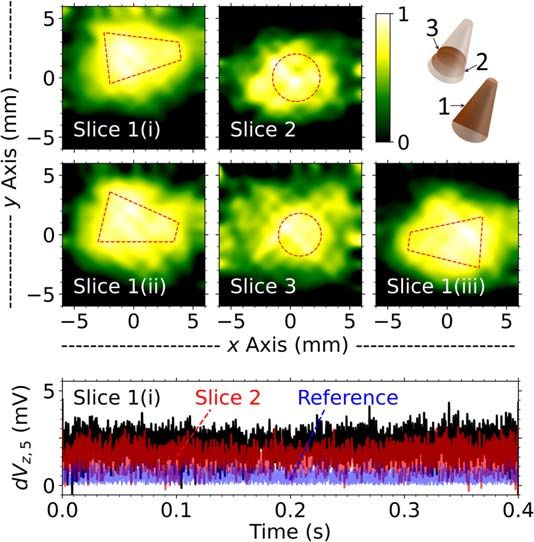
Appl. Phys. Express 14, 095001 (2021)                                                                                                       S. B. Trisnanto et al.

                                                                     (a)               terms of the sensitivity upon tracer mass (i.e. 4 mg iron
                                                                                       oxides) as compared to Ref. 24. The minimally imageable
                                                                                       sample mass of our prototype is 1 mg.
                                                                                          Regarding low sensitivity and poor spatial resolution of the
                                                                                       current MPI scanner, installing calibration coils or improving
                                                                                       receive coil and harmonic signal processing unit may
                                                                                       maximize MR sensor performance in MPI system.15) More
                                                                                       specifically, increasing turn number of impedance-matched
                                                                                       pickup and cancel coils, reducing ambient magnetic noise
                                                                                       level, and using narrow band-pass filter may be further
                                                                                       necessary. Although we currently focus on utilizing MR
         (b)
                                                                                       sensor, the strategy of using nonlinear properties to transform
                                                                                       monotone signal of the tracers into high order harmonic
                                                                                       signals can be potentially adopted for other nonlinear devices
                                                                                       and circuits. In this case, one may consider design simplicity
                                                                                       and careful signal processing in pursuit of high sensitivity
                                                                                       and high spatial resolution.
Fig. 5. (Color online) (a) Longitudinal and axial image slices of cone-                   In conclusion, we have demonstrated the applicability of
shaped solid ferucarbotran phantom. Slice 1 represents images longitudinally           MR sensor for extremely low field MPI, which exploits linear
taken at different positions and orientations: (i), (ii) and (iii), whereas slices 2   magnetization response of magnetic nanoparticles. We tech-
and 3 are circular axial cuts of the cone at different height. All images are
                                                                                       nically decompose odd harmonic components of the MR
normalized to each maximum pixel intensity. (b) Demodulated MPI signals
of slice 1(i) and 2. The slice area is proportional to dVz,5, where slice 1(i)         sensor output saturated by monotone magnetic signal from
(black line) has larger dVz,5 than slice 2 (red line); blue line is for sample-free    the receive coil. Under 40 μT/μ0 and 0.8 T m−1, the resulting
reference.                                                                             harmonic signals appears applicable to reconstruct high-
                                                                                       contrast images of the cone-shaped solid ferucarbotran
   In the case of modulated MPI, large trajectory density                              phantom with 4 mg iron oxide mass at frequencies below
optimized at fz/fx is crucial to fully cover field of view (FOV),                       the seventh order of the harmonics. To evaluate MR sensor
thus affecting spatial resolution.13) Low field gradient across                         performance, we further investigated different slices of the
the FOV and low excitation field cause poor image quality.23)                           phantom at fifth harmonic frequency, emphasizing SNR
Thus, 0.8 T m−1 and 40 μT/μ0, by default, produce poor                                 dependence of the imaged tracer area. Owing to its tunable
image obtained from direct dV0(x, y) plot (Fig. 4). For the                            saturation properties, MR sensor can be potential candidate
same situation, the MR sensor can provide high-contrast                                of magnetization sensing unit in the human-sized MPI
image because dVz,n(x, y) depends on Mz(t) instead of                                  system.
dMz(t)/dt [Eq. (2)] and the modulation ratio dVz,n/Vz,n                                   Acknowledgments This work was partially supported by the Japan
becomes larger than dV0/V0. Furthermore, high harmonic                                 Society for the Promotion of Science (JSPS) KAKENHI Grant No. 20H05652 and
                                                                                       the Standard Program of JSPS Postdoctoral Fellowship.
order of MR signal enables fine sampling of the FFP
                                                                                          ORCID iDs Suko Bagus Trisnanto      https://orcid.org/0000-0002-3440-
trajectory within the FOV, thus contributing to improving                              3460 Yasushi Takemura  https://orcid.org/0000-0003-3680-728X
spatial resolution. Nevertheless, MR signal distortion at n > 7
(Fig. 3) leads to a noisy image reconstructed at 9fz and 11fz.
Since the amplitude modulation is very sensitive to the image
                                                                                        1) B. Zheng, T. Vazin, P. W. Goodwill, A. Conway, A. Verma, E. U. Saritas,
processing, we require multiple signal filtering to further                                 D. Schaffer, and S. M. Conolly, Sci. Rep. 5, 14055 (2015).
exploit high-order harmonics of the MR sensor output.                                   2) P. Chandrasekharan et al., Theranostics 10, 2965 (2020).
However, we focus on utilizing n = 5 to analyze MR sensor                               3) P. Ludewig et al., ACS Nano 11, 10480 (2017).
performance in imaging the phantom (Fig. 5).                                            4) J. Rahmer, A. Antonelli, C. Sfara, B. Tiemann, B. Gleich, M. Magnani,
                                                                                           J. Weizenecker, and J. Borgert, Phys. Med. Biol. 58, 3965 (2013).
   Figure 5 discusses the capability of MR sensor to image                              5) H. Paysen, N. Loewa, A. Stach, J. Wells, O. Kosch, S. Twamley, M.
two different phantom slices: longitudinal and axial, at                                   R. Makowski, T. Schaeffter, A. Ludwig, and F. Wiekhorst, Sci. Rep. 10,
5fz = 50 kHz. In Fig. 5(a), the phantom shape is well                                      1922 (2020).
                                                                                        6) B. Gleich and J. Weizenecker, Nature 435, 1214 (2005).
preserved. For longitudinal slice 1, we imaged the phantom
                                                                                        7) J. B. Weaver, A. M. Rauwerdink, C. R. Sullivan, and I. Baker, Med. Phys.
while changing its orientation relative to the FOV. Slice 1(ii)                            35, 1988 (2008).
faces the same direction as slice 1(i) but with a more centered                         8) J. Weizenecker, B. Gleich, J. Rahmer, H. Dahnke, and J. Borgert, Phys.
position on the xy plane. We moved the sample mechanically                                 Med. Biol. 54, L1 (2009).
                                                                                        9) J. Rahmer, C. Stehning, and B. Gleich, PLoS One 13, e0193546 (2018).
by using a micrometer slider. We also flipped the sample
                                                                                       10) E. U. Saritas, P. W. Goodwill, G. Z. Zhang, and S. M. Conolly, IEEE Trans.
orientation to obtain slice 1(iii) which was able to preserve                              Med. Imaging 32, 1600 (2013).
the conical shape. However, slices 2 and 3 representing axial                          11) M. Graeser et al., Nat. Commun. 10, 1936 (2019).
cuts of the phantom appear blurry to visualize circular                                12) S. B. Trisnanto and Y. Takemura, Appl. Phys. Lett. 115, 123101 (2019).
                                                                                       13) S. B. Trisnanto and Y. Takemura, Phys. Rev. Applied 14, 064065 (2020).
pattern. Small imaged area is responsible for low SNR (i.e.                            14) R. Dhavalikar, L. Maldonado-Camargo, N. Garraud, and C. Rinaldi, J. Appl.
blurry effect) on the slices 2 and 3. Figure 5(b) further                                  Phys. 118, 173906 (2015).
confirms that signal intensity of slice 2 is indeed lower than                          15) Y. Adachi, D. Oyama, Y. Terazono, T. Hayashi, T. Shibuya, and
that of slice 1(i). The respective SNR of dVz,5 for recon-                                 S. Kawabata, IEEE Trans. Magn. 55, 8660661 (2019).
                                                                                       16) M. Graeser, T. Knopp, M. Grüttner, T. F. Sattel, and T. M. Buzug, Med.
structing slices 1(i) and 2 are 7.6 and 5.0 dB. Although these                             Phys. 40, 042303 (2013).
values are above the 3 dB threshold, they are relatively low in
                                                                               095001-4                         © 2021 The Japan Society of Applied Physics
Appl. Phys. Express 14, 095001 (2021) S. B. Trisnanto et al.
17) D. Pantke, N. Holle, A. Mogarkar, M. Straub, and V. Schulz, Med. Phys. 46, 21) P. W. Goodwill and S. M. Conolly, IEEE Trans. Med. Imaging 30, 1581
4077 (2019). (2011).
18) Y. Zhang, G. He, X. Zhang, and G. Xiao, Appl. Phys. Lett. 115, 022402 22) P. W. Goodwill, G. C. Scott, P. P. Stang, and S. M. Conolly, IEEE Trans.
(2019). Med. Imaging 28, 1231 (2009).
19) Z. W. Tay, D. W. Hensley, E. C. Vreeland, B. Zheng, and S. M. Conolly, 23) T. Sasayama, Y. Tsujita, M. Morishita, M. Muta, T. Yoshida, and
Biomed. Phys. Eng. Express 3, 035003 (2017). K. Enpuku, J. Magn. Magn. Mater. 427, 144 (2017).
20) H. Bagheri and M. E. Hayden, J. Magn. Magn. Mater. 498, 166021 (2020). 24) H. Paysen, O. Kosch, J. Wells, N. Loewa, and F. Wiekhorst, Phys. Med.
Biol. 65, 235031 (2020).
095001-5 © 2021 The Japan Society of Applied PhysicsYou can also read