Symmetry breaking in a turbulent environment
←
→
Page content transcription
If your browser does not render page correctly, please read the page content below
Symmetry breaking in a turbulent environment

                                                                                Alexandros Alexakis and François Pétrélis
                                                         Laboratoire de Physique de l’École Normale Supérieure, CNRS, PSL Research University,
                                                                     Sorbonne Université, Université de Paris, F-75005 Paris, France

                                                                                            Santiago J. Benavides
                                                                        Department of Earth, Atmospheric, and Planetary Sciences,
                                                                     Massachusetts Institute of Technology, Cambridge, MA 02139, USA

                                                                                          Kannabiran Seshasayanan
                                                  Service de Physique de l’Etat Condensé, CNRS UMR 3680, CEA Saclay, 91191 Gif-sur-Yvette, France and
                                                         Department of Physics, Indian Institute of Technology Kharagpur, Kharagpur 721 302, India
arXiv:2102.03618v1 [physics.flu-dyn] 6 Feb 2021

                                                                                          (Dated: February 9, 2021)
                                                         In this work we investigate symmetry breaking in the presence of a turbulent environment. The
                                                      transition from a symmetric state to a symmetry-breaking state is demonstrated using two examples:
                                                      (i) the transition of a two-dimensional flow to a three dimensional flow as the fluid layer thickness
                                                      is varied and (ii) the dynamo instability in a thin layer flow as the magnetic Reynolds number is
                                                      varied. We show that these examples have similar critical exponents that differ from the mean-field
                                                      predictions. The critical behavior can be related to the multiplicative nature of the fluctuations and
                                                      can be predicted in certain limits using results from the statistical properties of random interfaces.
                                                      Our results indicate the possibility of existence of a new class of out-of-equilibrium phase transition
                                                      controlled by the multiplicative noise.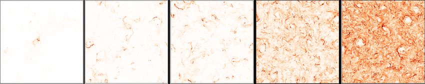
2

        FIG. 1. Vertical vorticity, ωz = ẑ · (∇ × u), of the 2D field for a random (left) and a turbulent state (right).

   Phase transitions are ubiquitous in nature. The liquid-gas transition or the transition from a magnetized to a
non-magnetized state in ferromagnetic materials are textbook examples [1–3]. Critical phenomena of continuous
phase transitions have been a major research topic for more than 50 years. It is now well understood that, at
equilibrium, the thermal fluctuations play a dominant role: the amplitude of the order parameter, say A, depends on
the distance from the critical point, say µ, as a power-law A ∝ µβ where the value of the exponent β differs from
the mean-field prediction obtained when thermal fluctuations are neglected. These results are verified in experiments
and are understood theoretically for instance through renormalization methods. In contrast, the behavior of critical
phenomena in non equilibrium systems remains less well understood. In liquid crystals, a transition between two
topologically different nematic phases was shown to belong to the class of directed percolation [4]. The transition
from the laminar state to turbulence in extended shear flows [5–7] is an out of equilibrium phase transition that also
belongs to the directed percolation universality class. Here we consider examples of bifurcations over a turbulent flow,
in which the system transitions from a state that respects a certain symmetry to a different state where this symmetry
is broken. We need to emphasise, that the transition is from a turbulent/chaotic state to an other turbulent state and
thus it differs from the classical laminar to turbulent transition. Furthermore, the symmetries and the nature of the
coupling of the turbulent fluctuations differ from the former examples indicating the possibility of a new universality
class.
   The first system that we consider is a two dimensional (2D) flow which undergoes an instability towards a three
dimensional (3D) flow. The nature of the transition from a 2D to a 3D flow is a challenging topic of wide-range
interest in turbulence [8]. It is a common situation in geophysics as rotation and the small pressure scale height of
planetary atmospheres tend to bidimensionalize the flows [9, 10]. Here we consider an idealized flow confined in a thin
layer of thickness H in the normal z-direction and of width L  H in the in-plane x and y directions with free slip
boundary conditions in z and periodic boundary conditions in x and y. The flow is described by the incompressible
velocity u that follows the Navier-Stokes equations,
                                         ∂t u + u · ∇u = −∇P + ν∇2 u − αu + f ,                                             (1)
  Where P is the pressure, ν is the kinematic viscosity and α is a drag coefficient that acts only on the vertically
averaged part of the flow, denoted by u, used to model Ekman friction [11]. Energy is injected by f a random delta-
correlated in time forcing, with a fixed averaged energy injection rate , an input parameter. It is two-dimensional,
depending only on x and y, so that f = f , and acts only on the horizontal components. It is acting at some length
scale `, such that H  `  L. The injection rate  and the length scale ` will be used to nondimensionalize our
system and will be set accordingly to unity. The part of the flow that varies along the vertical direction is denoted
as ũ = u − u and follows the equation
                                ∂t ũ + u · ∇ũ + ũ · ∇u = ũ · ∇ũ − ũ · ∇ũ − ∇P̃ + ν∇2 ũ.                             (2)
Note that because f = f the velocity variation ũ is not directly forced, so that ũ = 0 is always a solution of the
system. For very thin layers and close to the onset of the instability ũ can be approximated with one Fourier mode
in the z-direction as in [12].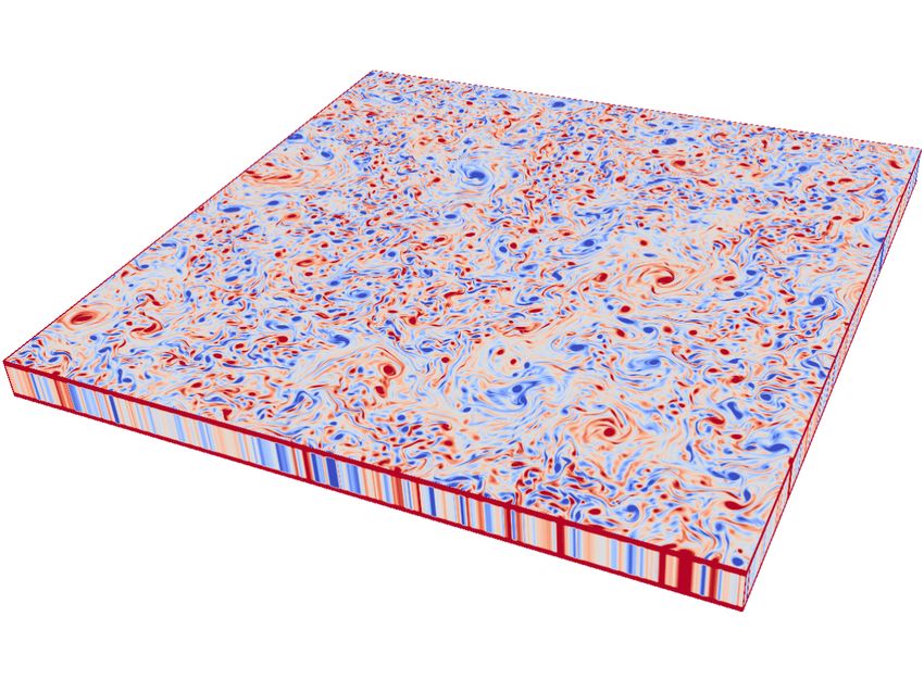
3

FIG. 2. First and second moment A1 , A2 for both the hydrodynamic problem and the MHD problem and for a random flow
and different values of Λ. The y-axis is normalised by A∗m = Am (3µc /2).

   For small H a purely two dimensional flow is generated, for which the velocity field is planar and invariant under
translation across the layer. Its dynamics is determined by the value of the Reynolds numbers Re = 1/3 `4/3 /ν and
Rα = 1/3 /α`2/3 . For small Re, Rα the flow is random following the statistical properties of the forcing with Gaussian
fluctuations, and a limited range of length-scales excited. In contrast, for large values of Re and Rα the flow is
turbulent and a cascade develops leading to fluctuations with non-Gaussian statistics distributed over a wide range of
scales. We will refer to these limiting cases as random and turbulent respectively. A snapshot of the vertical vorticity,
ωz = ẑ · (∇ × u), is displayed in Fig. 1 for a random (left panel) and a turbulent (right panel) state. In both cases, the
fluctuations do not depend on the vertical coordinate and the system is invariant in this direction ũ = 0. If however
H is increased, the flow breaks this symmetry and three-dimensional variations become unstable ũ 6= 0. The system
thus changes from a phase where ũ = 0 pointwise to a phase where ũ 6= 0 at a critical height that is shown to scale
like H ∝ `Re−1/2 [12]. In this system we use as control parameter µ the normalized height of the layer µ = H/` while
the order parameter is characterized by the different moments of the 3D fluctuations Am = h|ũ|m i where the angular
brackets stand for space-time-averaging. The size of the system is measured by the parameter Λ = L/`.
   The second system that we investigate is the dynamo instability of a swirling electrically conducting fluid tran-
sitioning from an unmagnetized to a magnetized state [13]. The system is governed by the equations of magneto-
hydrodynamics (MHD)

                                   ∂t u + u · ∇u = −∇P + ν∇2 u − αu + b · ∇b + f                                       (3)
                                                                 2
                                   ∂t b + u · ∇b = b · ∇u + η∇ b                                                       (4)

where b is the magnetic field and η the magnetic diffusivity. As in the previous case the considered flow is confined
in a thin layer, here with triple periodic boundary conditions. It is important to note that in the absence of the third
component no dynamo instability exists. For this reason, although the forcing is invariant along the z-direction as
before, all three components are present in f for this problem (i.e. two-dimensional, three-component, 2D3C). It is
again random and injects energy at a typical length ` at rate . The ratio of the energy injection rate in the transverse
component v to the energy injection rate in the in-plane directions h is measured by γ = v /h . The layer thickness
H is sufficiently thin so that the flow remains 2D3C u = u while it is thick enough so that a single Fourier mode of the
magnetic field becomes unstable b(x, y, z, t) = b̃(x, y, t)ei2πz/H as in [14, 15]. Keeping, Re, Rα , Λ (defined as before)
                                                                1/3
fixed we use the magnetic Reynolds number µ = Rm = h `4/3 /η as control parameter and as order parameter
the different moments of the magnetic field Am = h|b̃|m i. The two systems are numerically simulated using codes
described in [12, 15] on a 20482 grid. The simulations were run until a statistically steady state is reached in which
the different moments are measured.
   We begin by examining the random flow, for which Re ' Rα ' 1, depicted in the left panel of Fig. 1. The
amplitudes A1 and A2 are displayed in Fig. 2 as a function of µ for the hydrodynamic model (HD) and the MHD
model with γ = 4, for different values of Λ. For both systems the first and the second moment collapse on a
single master curve. Independence of the data on Λ also indicates that the large box limit has been reached. As a
consequence both systems appear to have the same critical behavior, suggesting a possibility that they belong to the
same universality class. The moments bifurcate from zero at a critical value µ = µc and scale with µ − µc as power
laws: A1 ∝ (µ − µc )β1 and A2 ∝ (µ − µc )β2 . An accurate estimate of the value of the exponents β1 , β2 is difficult to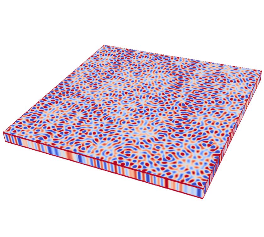
4
(a)
(b)
(c)
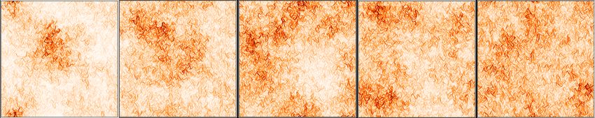
FIG. 3. For increasing values of µ (from left to right and starting from close to µc ) the images display (a) Energy density of
3D velocity field for the random base flow for the data points displayed in Fig. 2. (b) Energy density of the field φ for the field
equation, Eq. (5) with white noise solved on a 64 × 64 grid. (c) Energy density of magnetic field energy for the data points
displayed in Fig. 4.
obtain. For these turbulent systems, the existence of low frequency velocity fluctuations renders the situation difficult
as statistical convergence requires very long simulations. However, one can say with confidence that they clearly differ
from β1 = 1/2 and β2 = 1 that are the exponents obtained for static fields or by mean-field predictions where the
small scale fluctuations are modeled by tranport coefficients like an eddy diffusivity or an alpha coefficient [16]. They
also differ from the zero dimensional d = 0 bifurcations in the presence of multiplicative noise that is termed on-off
intermittency and leads to β1 = β2 = 1 [17, 18].
In order to explain these new exponents and to identify and characterize the universality class of these systems, we
resort to deriving a field equation, modeling the approximate equations of motion for the amplitude of the unstable
ũ and b near the threshold of instability. This derivation will be based on symmetries of the bifurcating system.
The hydrodynamic problem is symmetric under reflection in the z = 0 plane, which we denote by S. Once µ goes
beyond the critical value, the first linearly unstable vertical mode breaks this planar symmetry and is thus odd under
S. If we denote this solution ũ = φ(x, y, t)vu , where φ is the amplitude of the unstable mode and vu is the vertical
mode structure, then we have that Svu = −vu . Because the hydrodynamic problem is symmetric under reflection,
if φvu is a solution then Sφvu = −φvu is also a solution. In other words φ and −φ are solutions of the problem.
Similarly, for the magnetic problem, because of the invariance of the MHD equation under change of sign of the
magnetic field, if b is a solution so is −b. With the same reasoning let bu be the linearly unstable mode and φ its
amplitude, if φbu is a solution, so is −φbu . It is important to notice that these symmetries are satisfied even taking
into account the turbulent fluctuations. Therefore when modelling the effect of the turbulent fluctuations in the field
equation by stochastic terms, only odd terms in φ appear. Accordingly, the first order term in φ that couples to the
spatio-temporal fluctuations of the background field is linear. The symmetries of the problem thus imply that the
noise acting on the perturbation field is multiplicative. For the same reason, the lowest order nonlinear term is cubic.
We thus end with the following field equation
∂φ
= µφ − Cφ3 + D∇2 φ + ζ(x, t)φ (5)
∂t5 where ζ is spatio-temporal noise (interpreted in the Stratonovich sense), µ is the control parameter and C, D are constants. Here, the term ζ(x, t)φ expresses the local amplification or decrease effects, while µφ expresses their mean counter-parts. The non-linearity −Cφ3 is responsible for saturating the growth. The term D∇2 φ is responsible for diffusing any localized structure of φ. This equation has been studied to model for instance chemical reactions or synchronization transition [19–21]. When ζ is white and Gaussian, renormalization group methods allow to predict the critical behavior of the system. For a space of dimension d ≤ 2, a transition exists between an absorbing phase where φ = 0 and an active phase where φ 6= 0. Close to the critical point, the field scales as h|φ|n i = (µ − µc )βn . It has been shown [22] that some critical exponents of Eq. (5) can be related to the exponents of the Kardar-Parisi-Zhang equation (KPZ) [23, 24]. Indeed, the linear part of Eq. (5) is transformed by the Cole-Hopf transformation into the KPZ equation. This equation describes the growth of a random surface when nonlinear effects are taken into account. Some predictions of the KPZ equation are thus useful for the systems that we are considering. For d = 2 and white noise, the exponents βn have been calculated numerically β1 ' 1.14 and β2 ' 1.7 [25]. These predictions are displayed in Fig. 2 and are compatible with the results obtained for the two systems under study. The behavior of the different moments Am results from the spatial distribution of the unstable field (ũ, b, φ). In the top panels (a) of Fig. 3 five snapshots of the energy density of the field ũ are shown for different values of µ. The snapshots correspond to the data marked by blue diamonds in Fig. 2. Far from the onset (rightmost panels) the unstable field is spread throughout the domain. As µ comes closer to the onset the unstable field becomes more sparse occupying a smaller and smaller fraction of the domain. Very close to the onset (leftmost panel) only a few structures are left and in most of the domain the unstable field is almost zero. In panel (b) a series is shown for solutions of Eq. (5) that shows similar features. There are a few remarks that need to be made here. First we stress that the predictions for the field equation, Eq. (5), hold for the limit of infinite domain size Λ → ∞. For finite domains these exponents can be contaminated by finite size effects [26]. One can see for example from Eq. (5) that when the inverse diffusion time scale L2 /D is much smaller than the growth rate fluctuations, the spatial fluctuations are averaged out and the system recovers the mean field behavior. This limitation has a profound implications on the systems under study because the domain size is always finite and diffusion is controlled by eddy-diffusion that in general has non-trivial dependency with the system control parameters. For example, in the MHD system when we decrease the parameter γ we decrease the growth-rate that depends on the product of vertical and horizontal velocity components while we increase the turbulent diffusivity that depends only on the horizontal components. As a result the system becomes much more diffusive as γ is decreased. In Fig. 4 we show the behavior of A1 for the dynamo problem as in Fig. 2 but with a smaller value of γ = 1. The FIG. 4. Left panel: First moment A1 for the thin layer dynamo problem for γ = 1 for which turbulent diffusion is much more effective than in the case of Fig. 2. Right panel: First moment A1 for the thin layer problem for the turbulent flow. anomalous exponent observed in Fig. 2 is not present in the case of the left panel of Fig. 4 and the data are much better fitted with the mean field exponent β1 = 1/2. Similarly the second moment A2 (not plotted) here is much closer to β2 = 1. Finally, the energy distribution shown in panel (c) of Fig. 3 does not show the spatial distribution observed in the other panels. This observed mean-field behavior is however due to finite size effects. The anomalous scaling, and the associated intense localization of the field, are expected to be recovered in a larger system Λ → ∞. Furthermore, the predicted exponents based on Eq.(5) are valid when the noise is white. Their values differ when the noise has different properties (see for instance [24] p 285, and [27, 28]). Indeed when we simulate Eq.(5) with colored noise larger exponents are observed. The value of the measured exponents appeared to depend on the spectral
6

properties of the noise. This is important because in turbulent flows the spatio-temporal correlations of the fluctuations
are far from being white and Gaussian. In contrast to the random flow for which the fluctuations are localized in
scale, the energy cascade in the turbulent system leads to fluctuations across a wide range of scales. The exponents
measured for the fully turbulent flow, such as the one depicted in the right panel of Fig. 1, thus differ from the
predictions of Eq. (5) with a white noise. In the right panel of Fig. 4, A1 is displayed as a function of µ for the
hydrodynamic model in the turbulent state with Re ' 100, Rα ' 30 and for the same values of Λ as in Fig. 2. The
data overlap again in one master curve. The measured exponent is larger than both the mean field prediction and
the prediction of the white noise model of Eq. (5) and is closer to β1 ' 2. Theoretical predictions for Eq. (5) in 2D
with colored noise are still limited. Understanding the precise value of these exponents from properties of the KPZ
equations subject to colored spatio-temporal noise related to the spectral properties of turbulent flows would be of
great interest. Results for KPZ in 2D are still limited but in 1D, it is known that the roughness exponent (χ with the
notation of [22]) increases with the slope ρ of the noise spectrum (assumed to be of the form k −2ρ ). Assuming that this
remain true in 2D, and using the known scaling relations for the problem of multiplicative noise [22], we expect that
the exponent β is larger when ρ is large (for a turbulent flow and a noise term proportional to the velocity gradient
ρ = 1/3) than when the noise is white (ρ = 0) which has same exponent as in the case of the random flow. Thus the
exponent can be sensitive to the spatial properties of the turbulent fluctuations and in particular the existence of an
inverse cascade.
   Furthermore, the universality class can depend on the vectorial or scalar form of the bifurcating field [20]. In the
examined cases it is a vector for the two physical systems. For the field equation we have observed qualitatively
similar results for both a 2D vectorial and a scalar field. Further work and investigations are of course in order to
clarify if there are differences in this case too that could not be resolved by the present data.
   Finally we note that the considered systems are essentially 2D, and we expect that 3D systems belong to different
universality classes. Further investigations of field equations as Eq. (5) are required to determine the role of the
dimension of space and of the order parameter, as well as finite size effects and long-temporal and long-spatial noise
correlation effects. Further numerical but also experimental investigations are also indispensable for clarifying all
aspects of this transition. We believe that the results presented in this article open new directions for the study of a
variety of instabilities occurring over a turbulent system such as in turbulent atmospheric layers, surface waves driven
by turbulent winds in the ocean and magnetic dynamo field generation in stars driven by turbulent convection.

                                               ACKNOWLEDGMENTS

   This work was granted access to the HPC resources of MesoPSL financed by the Region Ile de France and the project
Equip@Meso (reference ANR-10-EQPX-29-01) of the programme Investissements d’Avenir supervised by the Agence
Nationale pour la Recherche and the HPC resources of GENCI-TGCC & GENCI-CINES (Project No. A0070506421)
where the present numerical simulations have been performed. This work has also been supported by the Agence
nationale de la recherche (ANR DYSTURB project No. ANR17-CE30-0004). SJB acknowledges funding from a grant
from the National Science Foundation (OCE-1459702).

 [1] S. K. Ma, Modern Theory of Critical Phenomena Frontiers in Physics (Reading, MA: Benjamin, 1976).
 [2] N. Goldenfeld, Lectures on Phase Transitions and the Renormalization Group Frontiers in Physics (Boulder, Co: Westview
     Press, 1992).
 [3] Jean Zinn-Justin, Quantum field theory and critical phenomena, Vol. 113 (Clarendon Press, Oxford, 2002).
 [4] Kazumasa A. Takeuchi, Masafumi Kuroda, Hugues Chaté, and Masaki Sano, “Directed percolation criticality in turbulent
     liquid crystals,” Phys. Rev. Lett. 99, 234503 (2007).
 [5] Grégoire Lemoult, Liang Shi, Kerstin Avila, Shreyas V Jalikop, Marc Avila, and Björn Hof, “Directed percolation phase
     transition to sustained turbulence in couette flow,” Nature Physics 12, 254 (2016).
 [6] Masaki Sano and Keiichi Tamai, “A universal transition to turbulence in channel flow,” Nature Physics 12, 249 (2016).
 [7] Matthew Chantry, Laurette S Tuckerman, and Dwight Barkley, “Universal continuous transition to turbulence in a planar
     shear flow,” Journal of Fluid Mechanics 824 (2017).
 [8] Alexandros Alexakis and Luca Biferale, “Cascades and transitions in turbulent flows,” Physics Reports 767, 1–101 (2018).
 [9] David Byrne and Jun A Zhang, “Height-dependent transition from 3-d to 2-d turbulence in the hurricane boundary layer,”
     Geophysical research letters 40, 1439–1442 (2013).
[10] Roland MB Young and Peter L Read, “Forward and inverse kinetic energy cascades in jupiter’s turbulent weather layer,”
     Nature Physics 13, 1135–1140 (2017).
[11] J. Pedlosky, Geophysical Fluid Dynamics (Springer-Verlag, 1987).
7
[12] Santiago Jose Benavides and Alexandros Alexakis, “Critical transitions in thin layer turbulence,” Journal of Fluid Mechanics
822, 364–385 (2017).
[13] H. K. Moffatt, Magnetic Field Generation in Electrically Conducting Fluids (Cambridge University Press, 1978).
[14] Kannabiran Seshasayanan and Francois Pétrélis, “Growth rate distribution and intermittency in kinematic turbulent
dynamos: Which moment predicts the dynamo onset?” EPL (Europhysics Letters) 122, 64004 (2018).
[15] Kannabiran Seshasayanan, Basile Gallet, and Alexandros Alexakis, “Transition to turbulent dynamo saturation,” Physical
review letters 119, 204503 (2017).
[16] Alexandros Alexakis, S Fauve, C Gissinger, and F Pétrélis, “Effect of fluctuations on mean-field dynamos,” Journal of
Plasma Physics 84 (2018).
[17] Hirokazu Fujisaka and Tomoji Yamada, “A new intermittency in coupled dynamical systems,” Progress of theoretical
physics 74, 918–921 (1985).
[18] NSEA Platt, EA Spiegel, and C Tresser, “On-off intermittency: A mechanism for bursting,” Physical Review Letters 70,
279 (1993).
[19] M.A. Munoz, “for a review see multiplicative noise in non-equilibrium phase transitions: a tutorial,” (2003).
[20] Uwe C Täuber, Critical dynamics: a field theory approach to equilibrium and non-equilibrium scaling behavior (Cambridge
University Press, 2014).
[21] Malte Henkel, Haye Hinrichsen, Sven Lübeck, and Michel Pleimling, Non-equilibrium phase transitions, Vol. 1 (Springer,
2008).
[22] Yuhai Tu, G. Grinstein, and M. A. Muñoz, “Systems with multiplicative noise: Critical behavior from kpz equation and
numerics,” Phys. Rev. Lett. 78, 274–277 (1997).
[23] Mehran Kardar, Giorgio Parisi, and Yi-Cheng Zhang, “Dynamic scaling of growing interfaces,” Phys. Rev. Lett. 56,
889–892 (1986).
[24] Timothy Halpin-Healy and Yi-Cheng Zhang, “Kinetic roughening phenomena, stochastic growth, directed polymers and
all that. aspects of multidisciplinary statistical mechanics,” Physics Reports 254, 215 – 414 (1995).
[25] Walter Genovese, Miguel A. Muñoz, and J. M. Sancho, “Nonequilibrium transitions induced by multiplicative noise,”
Phys. Rev. E 57, R2495–R2498 (1998).
[26] MN Barber, C Domb, and JL Lebowitz, “Finite-size scaling in phase transitions and critical phenomena,” edited by C.
Domb and JL Labors 8 (1983).
[27] F Pétrélis and A Alexakis, “Anomalous exponents at the onset of an instability,” Physical review letters 108, 014501
(2012).
[28] Alexandros Alexakis and François Pétrélis, “Critical exponents in zero dimensions,” Journal of Statistical Physics 149,
738–753 (2012).You can also read


