Operations and Maintenance for Multipurpose Offshore Platforms using Statistical Weather Window Analysis
←
→
Page content transcription
If your browser does not render page correctly, please read the page content below
Operations and Maintenance for
                  Multipurpose Offshore Platforms using
                  Statistical Weather Window Analysis
Taemin Heo∗ , Phong T. T. Nguyen† , Lance Manuel∗ , Maurizio Collu‡ , K A Abhinav‡ , Xue Xu‡ and Giulio Brizzi§
   ∗ Department  of Civil, Architectural and Environmental Engineering, University of Texas at Austin, Austin, Texas 78712
                                                   Email: taemin@utexas.edu
         † Faculty of Civil Engineering, HCMC University of Technology and Education, Ho Chi Minh City, Vietnam

                                                Email: phongnguyen@utexas.edu
     ‡ Department of Naval Architecture, Ocean & Marine Engineering, University of Strathclyde, Glasgow, UK G4 0LZ

                                               Email: maurizio.collu@strath.ac.uk
                                                   § Chlamys s.r.l., Trani, Italy

                                                    Email: chlamys@tiscali.it

   Abstract—With increasing offshore-related commerce, the          mix of crew transfer vessels (CTVs), service operation vessels
choice of appropriate operations and maintenance activities         (SOVs), and helicopters that transport specialized technicians.
must take into consideration safety, costs and performance          The feasibility of an O&M activity is assessed by comparing
targets. Stochastic weather conditions at each site of interest
presents uncertain situations. We present an optimized decision-    measured wave heights and wind speeds against operational
making procedure that seeks to maximize monetary benefits           capabilities of these transport systems. Differently, in the
while minimizing safety risks. Our proposed approach outlines       UK-China project, INNO-MPP (https://www.ukchn-core.com/
and illustrates application of such a policy by incorporating       project/inno-mpp/), where the feasibility of a wind-aquaculture
traditional weather window analysis using a Markov Decision         MPP at the same Scottish location discussed in this work
Process approach. In particular, the approach is applied in case
study involving the operation of a multipurpose platform at an      is considered [9], [10], it has emerged that the O&M of
offshore Scotland site.                                             aquaculture systems must usually rely on technicians who
                                                                    will decide about the acceptability of the metocean conditions
                      I. I NTRODUCTION                              based on more intuitive and human-readable metrics such as
   Weather conditions—e.g., wind speeds, wave heights,              the Beaufort scale, and not on, say, the measured significant
etc.—can vary greatly over the year at offshore sites. Off-         wave height, Hs . The O&M strategies adopted for such MPPs,
shore activities associated with operations and maintenance         then, have to take into account such human factors that can
(O&M) of multipurpose platforms (MPPs), see Fig. 1, for an          have a substantial impact on adopted policy.
example, are gaining in importance and often need different            With multipurpose platforms that are becoming increasingly
service activities periodically and/or under constraints to avoid   common in the “blue economy,” there is a need to be able to
downtime and loss of revenue (as with energy generation             deal with a wide-ranging set of operations related to the in-
from wind, waves, etc.). The literature contains examples           tended multiple uses [11]. An archived history of past weather
for dealing with O&M using weather windows in statistical           conditions at a selected site provides us with weather window
analyses—e.g., in aquaculture farming, offshore wind energy         statistics that can aid in a rational plan for O&M. Yet, a daily
generation, etc. These studies feature offshore sites around the    optimized decision-making guide, for not only minimizing
world including the Gulf of Mexico, the east and west coasts        down time and loss of revenue at the facility but also for
of Japan, the west coast of Ireland, the Barents Sea, the North     maximizing the safety of the operators, has not been systemat-
Atlantic Ocean, and the UK [1]–[6]. Reference [7] presented         ically studied. In the literature, some good examples of studies
a methodology for weather window prediction that considered         have been undertaken that involve the development of O&M
offshore vessels and challenges associated with operations in       decision models in wind energy applications. For instance,
Norway. Reference [8] evaluated the marine environment at a         References [12]–[14] employed a Partially Observed Markov
Korean wind farm to select appropriate O&M vessels.                 Decision Process (POMDP) to construct a stochastic model for
   One of the key driving factors for the long-term economical      quantifying risks and uncertainties, and developed an O&M
viability of MPPs, as for offshore renewable energy devices,        decision model for land-based wind turbines. Reference [15]
is accessibility: the ability to keep, for example, all renewable   reviewed many O&M decision support research studies for
energy systems, aquaculture systems, etc. operating. For off-       offshore wind farms. A reliability-based computational model
shore wind farms, accessibility is usually achieved through a       was also implemented to establish O&M procedures for an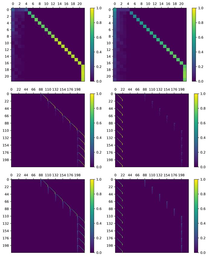
TABLE I
                                                                                          B EAUFORT W IND S CALE

                                                                          Beaufort      Wind Speed (m/s)        Wind Speed (m/s)
                                                                          Number            -Original-             -This Study-
                                                                             0                 < 0.5                  < 0.5
                                                                             1               0.5 − 1.5               0.5 − 1.5
                                                                             2               1.5 − 3.3               1.5 − 3.3
                                                                             3               3.3 − 5.5               3.3 − 5.5
                                                                             4               5.5 − 7.9               5.5 − 7.9
                                                                             5              7.9 − 10.7              7.9 − 10.7

             Fig. 1. Multipurpose Platform Concept [17].                     6              10.7 − 13.8            10.7 − 13.8
                                                                             7              13.8 − 17.1            13.8 − 17.1
                                                                             8              17.1 − 20.7            17.1 − 20.7
                                                                             9              20.7 − 24.4               ≥ 20.7
                                                                             10             24.4 − 28.4
                                                                             11             28.4 − 32.6
                                                                             12               ≥ 32.6

                                                                   C. O&M Decision Making Problem Setting
         Fig. 2. Temporal trends in mean wind speed at 10 m           We present next the problem formulation that addresses
                                                                   O&M decision making for offshore multipurpose platforms.
offshore renewable energy farm [16].                               There are different required work durations, tw , for the
   We propose, by using wind data from a Scottish site, how        different types of O&M activities involved. Based on the
a Markov Decision Process can be defined that facilitates          O&M vessels/equipment needed and the type of O&M activity,
rational decision-making while taking into consideration O&M       operable (acceptable) weather conditions are defined in terms
constraints as well as site-specific stochastic weather charac-    of maximum allowable Beaufort number, ξB . Then, from
teristics and the safety.                                          the data, we need to develop a time series, Xe (t), which
                                                                   represents favorable time segments with operable weather
               II. M ATERIALS AND M ETHODS                         conditions. Fig. 3 shows a illustrative example for an activity
A. Offshore Wind Speed Data                                        with ξB = 4 in January 2008. Triangular pulse-shaped time
   As far as weather conditions, this study considers the mean     segments increase while the Beaufort number is below the
wind speed at 10 m (v10 ) obtained every 6 hours, from 2008        threshold, ξB , and go to zero whenever the weather conditions
to 2017, at the location of a planned multipurpose platform        get more severe and exceed the threshold, ξB . When an
offshore Scotland (lat. 56.5◦ , lon. -7◦ ). Fig. 2 shows the v10   O&M activity needs to occurs at t0 , revenue starts to be lost
data, smoothed using a 30-day moving window for each year          after some time, taux , associated with some auxiliary system
separately. Seasonal patterns are clear; greater variability and   spending capacity. The per unit time loss of revenue is defined
more severe weather is evident in the winter. These stochastic     as cdown ; then, the loss at time t is cdown ∗max(D(t)−taux , 0),
characteristics of the weather serve to highlight the challenges   where D(t) is the down time (unavailable window) at time,
associated with dealing with it, while attempting to schedule      t. If Xe (t0 + tw ) = Xe (t0 ) + tw , the O&M activity can
and optimize O&M activities.                                       be successfully performed and the down time is reset to
                                                                   zero; otherwise, Xe (t0 + tw ) − Xe (t0 ) is less than tw , and
B. Beaufort Scale                                                  D(t0 + tw ) = D(t0 ) + tw indicating that the O&M activity
   For the weather window analysis, v10 can be related to the      was unsuccessful. In the latter case, a unit failure cost, cf ail , is
Beaufort scale, which is an empirical measure relating wind        charged. Successful and failed scenarios of an O&M activity
speed to observed conditions at sea and is widely used in          are illustrated in Fig. 3 with green and red shaded windows,
navigation and voyage forecasts. The original scale had 13         respectively. Possible changes of Xe (t) when Xe (t0 ) = i and
classes (going from 0 to 12), but this study uses only levels      tw = 3 (≡ 18 hours) are shown in Fig. 4.
0 to 9; levels greater than 9 are extreme observations and
account for only a small fraction of the data. Table 1 shows       D. Season Identification
the original Beaufort scale and the modified version used in         Fig. 2 provided an indication of seasonal variability in off-
this study.                                                        shore weather at the selected site. For simplicity, a stationary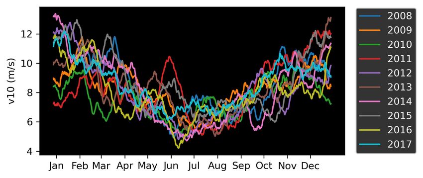
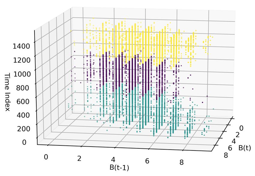
Fig. 5. Season identification result

                                                                                  study, it is more appropriate to discuss cost. At each discrete
Fig. 3. Example series of v10 , Beaufort scale, and favorable times of operable   time, the process is in state s ∈ S, while the decision maker
weather, Xe (t), where ξB = 4 with illustration of successful and failed          takes action a ∈ A and incurs cost R(s, a) as a result of the
scenarios of an O&M activity where tw = 3 (≡ 18 hours)
                                                                                  action. The process switches to a new state s0 according to a
                                                                                                                                          0
                                                                                  known stochastic model, with transition probability P (s |s, a).
                                                                                  The state transitions of an MDP satisfy the classical Markov
                                                                                  property:
                                                                                    P (st+1 |st , at , st−1 , at−1 , . . . , s0 , a0 ) = P (st+1 |st , at ). (1)
                                                                                  Then, the MDP helps to yield an optimized policy π ∗ (s).
                                                                                  The policy maps states to actions and the optimal policy is
                                                                                  iteratively found by exploring the best action for each state that
                                                                                  minimizes the overall cost function. Here, a discount factor γ,
                                                                                  0 ≤ γ ≤ 1, is introduced to account for present and future
                                                                                  value of relevant item. Dynamic programming, introduced by
Fig. 4. Possible cases of evolution of Xe where tw = 3 (i.e., required work
duration = 18 hours)
                                                                                  Bellman (1954), may be used to solve the MDP [18]. In this
                                                                                  study, to provide general guidelines that are independent of
                                                                                  time, we assume an infinite horizon problem and the value
stochastic weather process is assumed where each year is                          iteration is formulated as:
divided into two distinct periods. We are interested in the
                                                                                                           "
                                                                                                ∗             X
transition of the Beaufort number with time; accordingly, three                             V π (s) = max         P (s0 |s, a)R(s, a, s0 )+
                                                                                                          a∈A
variables, (B(t − 1),B(t),itime ), are used to define seasons                                                     s0 ∈S
                                                                                                                                                         #   (2)
by k-means clustering. B(t) is the Beaufort number at time t
                                                                                                                                              π∗
                                                                                                                       X
                                                                                                                                   0                 0
while itime is an annual 6-hour basis time index. Three clusters                                                   γ           P (s |s, a)V        (s )
with different colors are evident in Fig. 5. The transition time                                                       s0 ∈S

index can be inferred distinctly for each seasons as the clusters                 where V π is a value function that represents the expected
do not overlap. The purple cluster has benign conditions (low                     overall cost of policy π. The iterations terminate when the
Beaufort numbers), and its time index range is that of the                        difference between the value function in two consecutive steps
summer season, ranging from 490 (= 122.5 days = May 3rd)                          is below a specified level ε (more details can be found in [19]).
to 976 (= 244 days = Sep 1st).
                                                                                  F. Markov Decision Process Setting for the Problem
E. Markov Decision Process                                                           In the present study, there are only two actions, “Go” and
   A Markov Decision Process (MDP) is a discrete time                             “Stay”. The data are time-indexed every 6 hours. The range for
stochastic control process that can model situations where                        both favorable and down times is (0, ∞). In the finite discrete
outcomes are partly random and partly under the control of                        MDP process setting that we adopt, we limit this range for
a decision maker. An MDP is a 4-tuple (S, A, P, R) of state,                      favorable and down times. The maximum favorable and down
action, transition probability and cost (or reward). Reward is                    times are limited to 126 hours and 54 hours, respectively. For
common nomenclature in defining a MDP but, in the present                         convenience, a selected number of intervals is used to indicate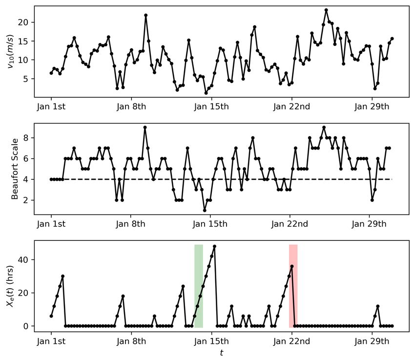
favorable and down times. As a result, the favorable times are
{0, 1, 2, . . . , 21} and down times are {0, 1, 2, . . . , 9}. Every
possible pair of favorable and down times is considered a state;
220 states are defined accordingly. An nth state indicates (n
mod 21) time steps of favorable time and a quotient (n/21)
time steps of down time. Transition probabilities are defined
using a matrix of dimension, 2 × 220 × 220 (resulting from
220 × 220 inter-state transition probabilities and two possible
actions at each state). Finally, the cost function is also defined
using a matrix of dimension, 220 × 2 (resulting from costs
incurred by the two actions for the 220 states).
   The transition probability matrix is constructed from the
data in two steps. First, an intermediate transition matrix of
favorable times is developed from Xe . A transition event from
Xe (t) = i to Xe (t + tw ) = i0 (where i0 ∈ {0, 1, ..., tw −
1, i + tw }) is monitored and each occurrence is counted and
included in the matrix of dimension, 22 × 22. By normalizing
this count-based matrix row by row, the intermediate transition
matrix results. Second, a reshaping of the matrix considering
actions and the down time, D(t), to yield the final transition
probability matrix for the MDP is needed. When the action
is “Stay”, D(t) will transition to D(t) + tw , regardless of
Xe (t) until D(t) + tw > 9 is true, since the consequence
of the action “Stay” is independent of the stochastic weather
process and we limit down time to 9 time steps (54 hours).
When D(t) + tw > 9, the down time is assumed to stay at
9. The action “Go” results in two scenarios. When the O&M
activity is successful—i.e., Xe (t+tw ) = Xe (t)+tw and D(t+           Fig. 6. Algorithms for constructing transition probability matrix and cost
tw ) → 0. If there was at least one bad weather—i.e., Xe (t +          matrix
tw ) < tw , then the O&M activity is assumed to have failed and
D(t + tw ) = D(t) + tw . Algorithms 1 and 2 in Fig. 6 indicate
the two steps in the transition probability matrix construction
procedure; Fig. 7 shows the structure of the transition matrix.
   A cost matrix is constructed next. For each action “Stay”,
cdown is charged for every state that has longer down time than
taux . For each action “Go”, cdown is also charged for every
state that has longer down time than taux . Additionally, cf ail
is charged for states with more severe weather than ξB . For
states that indicate successful O&M activity—i.e., zero down
time—no cost is charged. Algorithm 3 in Fig. 6 shows how
the cost matrix is constructed while Fig. 7 shows the structure
of the cost matrix.

                      III. A C ASE S TUDY

   A case study with ξB = 5, tw = 4, taux = 2, cdown = −1.5,
and cf ail = −1 is considered and the constructed transition
matrices are shown in Fig. 8. Note that taux = 2 means that
for the O&M activity of interest, a loss of revenue results after
2 time steps (12 hours) of unfavorable weather; a duration of
4 time steps (24 hours) of favorable weather with Beaufort             Fig. 7. Structure of the transition matrix and the cost matrix when tw = 2
                                                                       (≡ 12 hours), taux = 1 (≡ 6 hours)
number not greater than 5 is needed for this O&M activity.
The cost associated with lack of use (down time) is 1.5 times
higher than the cost of failure. As a result of the value iteration,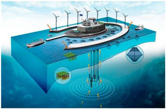
Fig. 8. Constructed intermediate transition matrix Asummer (upper left), Awinter (upper right), final transition matrix elements Pstay
                                                                                                                                  summer (center left),
Pgo                       stay                  go
  summer (center right), Pwinter (lower left), Pwinter (lower right).
the policy is optimized as follows: [7] T. Gintautas and J. D. Sørensen, “Improved methodology of weather
( window prediction for offshore operations based on probabilities of
0, (s mod 21) ≤ 1 operation failure,” Journal of Marine Science and Engineering, vol. 5,
∗
πsummer (s) = no. 2, p. 20, 2017.
1, Otherwise [8] D. Ahn, S.-C. Shin, S.-Y. Kim, H. Kharoufi, and H.-C. Kim, “Compar-
( (3) ative evaluation of different offshore wind turbine installation vessels
∗ 0, (s mod 21) ≤ 3 for korean west–south wind farm,” International Journal of Naval
πwinter (s) = Architecture and Ocean Engineering, vol. 9, no. 1, pp. 45–54, 2017.
1, Otherwise [9] K. Abhinav, M. Collu, S. Ke, and Z. Binzhen, “Frequency domain
analysis of a hybrid aquaculture-wind turbine offshore floating system,”
From the results, one can infer that, in the summer, a duration in 37th International Conference on Ocean, Offshore and Arctic Engi-
of favorable time of operable weather longer than 2 time steps neering, ASME, Glasgow, Scotland, June 2019.
(12 hours) indicates a “Go” action to do the O&M activity [10] K. A. Abhinav, X. Xu, Z. Lin, and M. Collu, “Dynamic response of a
multi-purpose floating offshore structure under extreme sea conditions,”
is recommended. In the more severe weather conditions and in International Conference on Ships and Offshore Structures ICSOS
greater variability in the stochastic weather process in the 2020, Glasgow, Scotland, September 2020.
winter, a duration of favorable time of operable weather longer [11] M. Vierros and C. De Fontaubert, “The potential of the blue economy:
increasing long-term benefits of the sustainable use of marine resources
than 4 time steps (24 hours) is needed to recommend “Go”. for small island developing states and coastal least developed countries,”
This optimized policy is independent of the down time since The World Bank, Tech. Rep., 2017.
cdown is assumed constant; however, loss of revenue varies [12] E. Byon, L. Ntaimo, and Y. Ding, “Optimal maintenance strategies
for wind turbine systems under stochastic weather conditions,” IEEE
linearly with down time. In some situations, the loss in revenue Transactions on Reliability, vol. 59, no. 2, pp. 393–404, 2010.
may be exponential with down time or, as for a fish farm, [13] E. Byon and Y. Ding, “Season-dependent condition-based maintenance
cdown may be a function of down time; then, an optimized for a wind turbine using a partially observed markov decision process,”
IEEE Transactions on Power Systems, vol. 25, no. 4, pp. 1823–1834,
policy will be dependent on down time. In another scenario, it 2010.
is possible that favorable weather is indicated and its duration [14] E. Byon, “Wind turbine operations and maintenance: a tractable approx-
exceeds 21 time steps; then, a “Go” action is recommended imation of dynamic decision making,” IIE Transactions, vol. 45, no. 11,
pp. 1188–1201, 2013.
at the site due to highly stationary weather. [15] H. Seyr and M. Muskulus, “Decision support models for operations
and maintenance for offshore wind farms: A review,” Applied Sciences,
IV. C ONCLUSION vol. 9, no. 2, p. 278, 2019.
[16] G. Rinaldi, P. Thies, R. Walker, and L. Johanning, “A decision support
This study proposed a framework to develop an O&M model to optimise the operation and maintenance strategies of an
strategy for multipurpose offshore platforms. The approach offshore renewable energy farm,” Ocean Engineering, vol. 145, pp. 250–
describes an optimized decision making policy given stochas- 262, 2017.
[17] Y.-T. Sie, P.-A. Château, Y.-C. Chang, and S.-Y. Lu, “Stakeholders
tic weather data, as well as O&M activity and cost constraints. opinions on multi-use deep water offshore platform in Hsiao-Liu-Chiu,
Exhaustive evaluation of all scenarios is possible using a taiwan,” International Journal of Environmental Research and Public
Markov Decision Policy framework that can be employed in Health, vol. 15, no. 2, p. 281, 2018.
[18] R. Bellman, “The theory of dynamic programming,” Rand Corp. Santa
planned blue economy projects. Monica CA, Tech. Rep., 1954.
[19] K. G. Papakonstantinou and M. Shinozuka, “Planning structural inspec-
ACKNOWLEDGMENT tion and maintenance policies via dynamic programming and markov
processes. Part I: Theory,” Reliability Engineering & System Safety, vol.
The 4th, 5th, and 6th authors are supported by the UK 130, pp. 202–213, 2014.
Engineering and Physical Sciences Research Council UK
(EPSRC) and the Natural Environment Research Council UK
(NERC), through Grants EP/R007497/1 and EP/R007497/2,
and the Natural Science Foundation of China (NSFC) through
Grant 51761135013.
R EFERENCES
[1] M. Du, J. Yi, P. Mazidi, L. Cheng, and J. Guo, “An approach for evalu-
ating the influence of accessibility on offshore wind power generation,”
Preprints, 2017.
[2] Y. Kikuchi and T. Ishihara, “Assessment of weather downtime for the
construction of offshore wind farm by using wind and wave simulations,”
in Journal of Physics: Conference Series, vol. 753, 2016, p. 092016.
[3] M. O’Connor, T. Lewis, and G. Dalton, “Weather window analysis of
irish west coast wave data with relevance to operations & maintenance
of marine renewables,” Renewable energy, vol. 52, pp. 57–66, 2013.
[4] A. Orimolade and O. Gudmestad, “On weather limitations for safe
marine operations in the barents sea,” in IOP Conf. Ser. Mater. Sci.
Eng, vol. 276, 2017, p. 012018.
[5] D. Martins, G. Muraleedharan, and C. Guedes Soares, “Analysis on
weather windows defined by significant wave height and wind speed,”
Renewable Energies Offshore, vol. 91, 2015.
[6] J. Paterson, F. D’Amico, P. Thies, R. Kurt, and G. Harrison, “Offshore
wind installation vessels–a comparative assessment for uk offshore
rounds 1 and 2,” Ocean Engineering, vol. 148, pp. 637–649, 2018.You can also read