Viable Medical Waste Chain Network Design by Considering Risk and Robustness
←
→
Page content transcription
If your browser does not render page correctly, please read the page content below
Viable Medical Waste Chain Network Design by Considering Risk and Robustness Reza Lot ( reza.lot .ieng@gmail.com ) Yazd University https://orcid.org/0000-0001-5868-8467 Bahareh Kargar Iran University of Science and Technology Alireza Gharehbaghi Sharif University of Technology Gerhard-Wilhelm Weber Poznan University of Technology: Politechnika Poznanska Research Article Keywords: Viable, Medical waste, Network design, Resiliency, Sustainable, Robust optimization Posted Date: August 17th, 2021 DOI: https://doi.org/10.21203/rs.3.rs-765430/v1 License: This work is licensed under a Creative Commons Attribution 4.0 International License. Read Full License
1 Viable medical waste chain network design by considering
2 risk and robustness
3 Reza Lotfi a, Bahareh Kargar b, Alireza Gharehbaghi c,
4 Gerhard-Wilhelm Weber d
a
5 Department of Industrial Engineering, Yazd University, Yazd, Iran and Behineh Gostar Sanaye
6 Arman, Tehran, Iran;
b
7 School of Industrial Engineering, Iran University of Science and Technology, Tehran, Iran;
c
8 Department of Industrial engineering, Sharif University of Technology, Iran;
d
9 Poznan University of Technology, Faculty of Engineering Management, Poznan, Poland, and
10 IAM, METU, Ankara, Turkey.
11
12 Abstract
13 Medical Waste Management (MWM) is an important and necessary problem in the COVID-19
14 situation for treatment staff. When the number of infectious patients grows up and amount of
15 MWMs increases day by day. We present Medical Waste Chain Network Design (MWMCND)
16 that contains Health Center (HC), Waste Segregation (WS), Waste Purchase Contractor (WPC)
17 and landfill. We propose to locate WS to decrease waste and recover them and send them to the
18 WPC. Recovering medical waste like metal and plastic can help the environment and return to the
19 production cycle. Therefore, we proposed a novel Viable MWCND by a novel two-stage robust
20 stochastic programming that considers resiliency (flexibility and network complexity) and
21 sustainable (energy and environment) requirements. Therefore, we try to consider risks by
22 Conditional Value at Risk (CVaR) and improve robustness and agility to demand fluctuation and
23 network. We utilize and solve it by GAMS CPLEX solver. The results show that by increasing the
24 conservative coefficient, the confidence level of CVaR and waste recovery coefficient increases
25 cost function and population risk. Moreover, increasing demand and scale of the problem make to
26 increase the cost function.
27
28 Keywords: Viable; Medical waste; Network design; Resiliency; Sustainable; Robust
29 optimization.
30
reza.lotfi.ieng@gmail.com;
1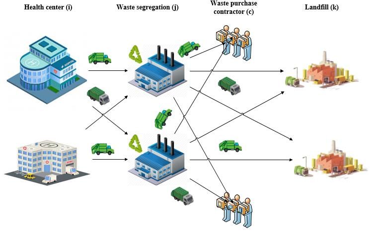
31   1. Introduction
32   Medical Waste Management (MWM) is a critical problem in the COVID-19 situation. In the
33   COVID-19 condition, amount of infectious patients grow up and amount of MWMs increase. As
34   a result, we must pay more attention to MWMs and improve waste disposal. Many workers that
35   do waste disposal, this subject threatens them very much. MWMs include infectious waste,
36   hazardous waste, radioactive waste and general waste (municipal solid waste). The WHO classifies
37   medical waste into sharps, infectious, pathological, radioactive, pharmaceuticals, other (including
38   toilet waste produced at hospitals). About 85% of MWMs are general waste and 15% of MWMs
39   are infectious waste, hazardous waste, radioactive waste (Tsai, 2021). Therefore, the importance
40   of MWMs, make many researchers contribute this subject and present mathematical approach and
41   decision support system. Some researchers consider a location-routing problem for medical waste
42   management (Suksee & Sindhuchao, 2021; Tirkolaee, Abbasian, & Weber, 2021). Others
43   investigate reverse logistics by the mathematical model (Sepúlveda, Banguera, Fuertes, Carrasco,
44   & Vargas, 2017; Suksee & Sindhuchao, 2021). Also, some scientists analysis of MWM systems
45   by multi-criteria-decision approach (Aung, Luan, & Xu, 2019; Narayanamoorthy et al., 2020). The
46   objective of these tools is to improve waste management performance and decrease risks for
47   workers that we can see in Figure 1.

                                 Figure 1. MWM in the COVID-19 situation.

                                                     2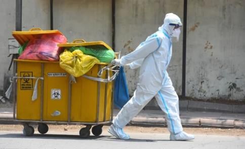
48 One of the new discussions in the present age is the viability of network design in post-pandemic
49 adaptation. The viability of networks that are proposed by Ivanov and Dolgui (2020) is integrated
50 agility, resilience and sustainability in the network. Therefore, it is needed to suggest a systematic
51 and mathematical model for setting up Viable Medical Waste Chain Network Design
52 (VMWCND). Because improving the performance of waste management is urban need and make
53 to prevent COVID-19 outbreak. Eventually, we should design a new mathematical model to
54 consider agility, resilience, sustainability, risks and robustness to cope with environmental
55 requirements and disruption.
56 Eventually, the innovation of this research and the main objective is as follows:
57 First time designing viable medical waste chain network design (VMWCND),
58 Considering robustness and risk in VMWCND.
59 The paper is organized as follows. In Section 2, we survey on related work in scope of MWCND.
60 In Section 3, the VMWCND and risk-averase VMWCND is stated. In Section 4, the results of
61 research and sensitivity analysis are presented. In Section 5, the managerial insights and practical
62 implications is discussed. In Section 6, the conclusion is summarized.
63 2. Survey on recent MWCND
64 The amount of waste has increased because of the COVID-19 situation. Therefore, researchers
65 research to manage, improve and decrease losses from medical centers. We survey on the recent
66 investigation on MWCND is as follows.
67 Mantzaras and Voudrias (2017) considered an optimization model for medical waste in Greece.
68 They tried to minimize total cost include location and transfer between location. The Genetic
69 Algorithm (GA) is applied to solve the model. Budak and Ustundag (2017) designed a reverse
70 logistic for multiperiod, multitype waste products. The model's objective was to minimize total
71 cost and the model's decision included location, flow, inventory. The case was in Turkey. They
72 found that by increasing waste amounts, the numbers of facilities and strategies are changed.
73 Wang, Huang, and He (2019) designed a two-stage reverse logistics network for urban healthcare
74 waste with multi-objective and multi-period. In stage one, they predicted the amount of medical
75 waste, and in the second stage, they minimized total cost and environmental impact.
376 Kargar, Paydar, and Safaei (2020) presented a reverse supply chain for medical waste. They used
77 mix-integer programming (MIP) to model problem. The objectives included total costs, technology
78 selection and the total medical waste stored that are minimized. A robust possibilistic
79 programming (RPP) approach are applied to cope with uncertainty. A Fuzzy Goal Programming
80 (FGP) method is embedded to solve the objectives. The real case study is investigated in Babol,
81 Iran. Other works of Kargar, Pourmehdi, and Paydar (2020) studied a reverse logistics network
82 design for MWM in the COVID-19 situation. They minimized the total costs, transportation and
83 treatment MW risks, and maximized the amount of uncollected waste. They employed the Revised
84 Multi-Choice Goal Programming (RMGP) method. Homayouni and Pishvaee (2020) surveyed
85 hazardous hospital waste collection and disposal network design problem with a bi-objective
86 robust optimization (RO) model. The objectives include total costs, the total operational and
87 transportation risk. An augmented ε‑constraint (AUGEPS) method is embedded to solve the
88 problem. The real case study is investigated in Tehran, Iran.
89 Yu, Sun, Solvang, and Zhao (2020) considered a reverse logistics network design for MWM in
90 epidemic outbreaks in Wuhan (China). The objectives included risk at health centers, risk related
91 to the transportation of medical waste and total cost. They solved the model by Fuzzy
92 Programming (FP) approach for multi-objective. They determine temporary transit centers and
93 temporary treatment centers in their model. In addition, Yu, Sun, Solvang, Laporte, and Lee (2020)
94 studied a stochastic network design problem for hazardous WM. They minimized cost and
95 transportation cost of hazardous waste and the population exposure risk. They applied stochastic
96 programming with Sample average approximation (SAA) for scenario reduction. They solved the
97 model by Goal Programming (GP). Z Saeidi-Mobarakeh, R Tavakkoli-Moghaddam, M
98 Navabakhsh, and H Amoozad-Khalili (2020) presented bi-level programming (BP) for a hazardous
99 WM problem. They used an enviormental approach for upper-level and routing and cost for lower-
100 level. They solve Mix-Integer Non-Linear Programming (MINLP) by GA.
101 In addition, Zahra Saeidi-Mobarakeh, Reza Tavakkoli-Moghaddam, Mehrzad Navabakhsh, and
102 Hossein Amoozad-Khalili (2020) developed a robust bi-level optimization model to model
103 hazardous WCND. They suggested a robust optimization approach to cope with the uncertainty.
104 Also, the decisions of the model include location, determining capacity and routing. Eventually, a
105 commercial solver is utilized to solve the model. Tirkolaee et al. (2021) surveyed a sustainable
4106 fuzzy multi-trip location-routing problem for MWM during the covid-19 outbreak. They
107 embedded Fuzzy Chance-Constrained Programming (FCCP) technique to tackle the uncertainty.
108 Therefore, they implemented Weighted GP (WGP) method to analyze and solve the problem. A
109 case study is determined in Sari, Iran to show the performance of the proposed model. Tirkolaee
110 and Aydın (2021) suggested a sustainable MWM for collection and transportation for pandemics.
111 They minimized total cost and the total risk exposure imposed by the collection. Eventually, a
112 commercial solver is utilized to solve the model with Meta-Goal Programming (MGP) for multi-
113 objective. Shadkam (2021) designed a reverse logistics network for COVID-19 and vaccine waste
114 management. They utilized Cuckoo Optimization Algorithm (COA). They tried to minimize total
115 cost. Nikzamir, Baradaran, and Panahi (2021) suggested a location routing network design for
116 MWM that tried to minimize the total cost and risks of population contact with infectious waste.
117 They offered a Mix-Integer Linear Programming (MILP) and solved it by a hybrid meta-heuristic
118 algorithm based on Imperialist Competitive Algorithm (ICA) and GA. Li et al. (2021) surveyed a
119 Vehicle Routing Problem (VRP) for MWM by considering transportation risk. They suggested MILP for
120 time window VRP and developed a Particle Swarm Optimisation (PSO) algorithm to solve large-scale
121 problems.
Table 1. Survey of MWCND.
Objectives
Uncertainty
Environmental
Economic
Case
Energy
Social
others
Reference Kind Decsion Methodology
study
(Mantzaras
Location,
& Voudrias, - - - - - MILP+ GA - Greece
capacity
2017)
(Budak & Location,
Ustundag, - flow, - - - - MILP - Turkey
2017) inventory
(Wang et al., Location,
Shanghai,
Green flow, - - - MILP -
2019) China
inventory
(Kargar, Location,
Babol,
Paydar, et - flow, - - - MILP+ FGP RPP
Iran
al., 2020) inventory
(Kargar,
Location,
Pourmehdi, - - - - MILP+RMGP - Iran
flow
et al., 2020)
(Homayouni
Location, MILP+ Tehran,
& Pishvaee, - - - - RO
flow AUGEPS Iran
2020)
5(Yu, Sun,
Location, Wuhan,
Solvang, & - - - - MILP+FP -
flow China
Zhao, 2020)
(Yu, Sun,
Numerical
Solvang, Location,
- - - - MILP+GP Stocastic example
Laporte, et flow
(NE)
al., 2020)
(Z Saeidi- Routing,
MINLP Isfahan,
Mobarakeh - environmenta - - - -
(BP)+GA Iran
et al., 2020) l
(Zahra
Location,
Saeidi- Isfahan,
- capacity, - - - MILP (BP) RO
Mobarakeh Iran
routing
et al., 2020)
(Tirkolaee
Location,
Sustainable - - - - MILP+WGP FCCP Sari, Iran
et al., 2021) routing
(Tirkolaee
& Aydın, Location,
Sustainable - - - MILP+ MGP - NE
routing
2021)
(Shadkam, Location,
- - - - - MILP + COA - NE
2021) flow
(Nikzamir Location, MILP+ICA,
Green - - - - NE
et al., 2021) routing GA
(Li et al.,
- Routing - - - - MILP + PSO - NE
2021)
Viable
This (Resilience Location, RO
- - - - MILP Tehran
research +sutainable flow Stochastic
+agile)
122 The classification of the literature is addressed in Table 1. It can be seen; researchers do not survey
123 the VMWCND problem. This study investigates the VMWCND problem and used mathematical
124 problems to locate the best place for MWCND.
125 The main innovation of this research is as follows:
126 First time designing VMWCND,
127 Considering agility, resilience, sustainability, robustness and risk-averse.
128 3. Problem description
129 In this research, we try to design VMWCND. The previous section shows a lack of research in
130 resilience, sustainability and agility MWCND. In the present study, we have Health Center (HC),
131 Waste Segregation (WS), Waste Purchase Contractor (WPC), landfill that waste move through
132 this network. Eventually, we present VMWCND through resilience strategy (flexible and scenario-
133 based capacity and node complexity), sustainability constraints (energy and environmental
6134 pollution), and agility (balance flow and demand satisfaction). We need to locate WS to improve
135 and recover waste and consider sustainability and environmental requirements in this situation.
136 Assumptions:
137 All wastes should be transferred to HC (agility),
138 All forward MWCND constraints include flow and capacity constraint is active,
139 Sustainability constraints include allowed emission and energy consumption are added
140 (sustainability),
141 Flexible capacity for facilities and node complexity in WS is considered as a resilience
142 strategy (resiliency),
143 Using scenario-based robust optimization against risks (robustness, risk, resiliency)
144 (Ivanov, 2020; Lotfi, Mehrjerdi, Pishvaee, Sadeghieh, & Weber, 2021).
Figure 2. Viable medical waste chain network design (VMWCND).
145 Notations:
146 Indices:
7i Index of Health Center (HC) i ,
j Index of Waste Segregation (WS) j ,
c Index of Waste Purchase Contractor (WPC) c ,
k Index of landfill k ,
t Index of time period,
s Index of scenario;
147 Parameters:
ww its Waste generated in HC i for time period t under scenario s ,
vij ijts Variable cost from HC i to WS j for time period t under scenario s ,
vjc jcts Variable cost from WS j to WPC c for time period t under scenario s ,
vjk jkts Variable cost from WS j to the landfill k for time period t under scenario s ,
fj j Cost of activation WS j ,
Emij ijts Emission CO2 for transfering from HC i to WS j for time period t under
scenario s ,
Emjc jcts Emission CO2 for transfering from WS j to WPC c for time period t under
scenario s ,
Emjk jkts Emission CO2 for transfering from WS j to landfill k for time period t under
scenario s ,
Enij ijts Energy consumption for transfering from HC i to WS j for time period t under
scenario s ,
8Enjc jcts Energy consumption for transfering from WS j to WPC c for time period t under
scenario s ,
Enjk jkts Energy consumption for transfering from WS j to landfill k for time period t
under scenario s ,
Capj jts Capacity WS j for time period t under scenario s ,
ps Probably of scenario s ,
Coefficient of conservative,
EMSC ts Maximum allowed emission for time period t under scenario s ,
ENSC ts Maximum allowed energy consumption for time period t under scenario s ,
j Coefficient of availability of WS j ,
Mbig Big positive number,
eps Very little positive number,
The confidence level for conditional value at risk,
Waste recovery coefficient,
TT Threshold of node complexity for resiliency,
The ratio of HC to WS.
popij ijts Population risk contact from HC i to WS j for time period t under scenario s ,
popjc jcts Population risk contact from WS j to WPC c for time period t under scenario s ,
popjk jkts Population risk contact from WS j to landfill k for time period t under scenario
s;
148 Decision variables:
149 Binary variables:
9xj If WS j is established, equal 1; otherwise 0;
150 Continues Variables:
wij ijts Waste transshipment from HC i to WS j for time period t under scenario s ,
wjk jkts Waste transshipment from WS j to landfill k for time period t under scenario s ,
wjc jcts Waste transshipment from WS j to WPC c for time period t under scenario s ;
151 Auxiliary Variables:
FC Fix cost of establishing WS
VCs Variable cost for scenario s ,
s Fix cost and variable cost for scenario s .
VaR Value at Risk
Auxiliary variable for linearization max function,
yij ijts Auxiliary and binary variable for linearization sign function for wij ijts ,
yjk jkts Auxiliary and binary variable for linearization sign function for wjk jkts ,
yjc jcts Auxiliary and binary variable for linearization sign function for wjc jcts .
152 3.1. VMWCND mathematical model
max(s ) CV aR (1 ) ( s )
minimize Z (1 ) p s s ( ) (1)
s 2
subject to:
s FC VC s , (2)
FC fj j x j , (3)
j
10VC s (vij ijtswij ijts vjk jktswjk jkts vjc jctswjc jcts ), s (4)
t i j j k j c
Agility constraints (flow constraints):
wij
j
ijts ww its , i , t , s (5)
wij
j
ijts wjk jkts wjc jcts ,
j j
i , k , c , t , s (6)
wij
i
ijts wjk jkts wjc jcts ,
k c
j , t , s (7)
wjk
k
jkts (1 )wij ijts ,
i
j , t , s (8)
Resiliency constraints (flexible and scenario-based capacity and node complexity)
wjk
k
jkts wjc jcts j Capj jts x j ,
c
j , t , s (9)
x j
, (10)
j
i
wij
i
ijts wjk jkts wjc jcts TT ,
k c
j , t , s (11)
Sustainability constraints (allowed emission and energy consumption):
Emij
i j
ijts wij ijts Emjk jktswjk jkts
j k
t , s (12)
Emjc jctswjc jcts EMSC ts ,
j c
Enij
i j
ijts wij ijts Enjk jktswjk jkts
j k
t , s (13)
Enjc jctswjc jcts ENSC ts ,
j c
11Pop s ( popij ijts wij ijts popjk jkts wjk jkts
t i j j k
s (14)
popjc jcts wjc jcts ),
j c
p Pop
s
s s , (15)
Decision variables:
x j {0,1}, j (16)
wij ijts ,wjk jkts ,wjc jcts 0. i , j , c ,
(17)
k ,t , s
153 The objective (1) considered minimizing the weighted expected value, minimax and conditional
154 value at risk of the cost function and for all scenarios. This form of the cost function is proposed
155 for robustness and risk-averse against disruption with worst condition. Constraints (2) include fix
156 and variable costs. Constraints (3) show fix-costs that include fix-cost activating WS for all
157 periods. Constraints (4) indicate the variable costs of HC, WS, WPC and landfill. Constraints (5)
158 show waste transshipment from HC to WS. Constraints (6) to (7) are flow constraints in forwarding
159 VMWCND. Constraints (8) determine the ratio of waste that goes to the landfill. Constraints (9)
160 are flexible capacity constraints for WS that less than the capacity of WS system. Constraints (10)
161 are resilience constraints and the number of WS is greater than the coefficient of HC. Constraints
162 (11) are resilience constraints and show node complexity in WS that summation of input and output
163 of every WS is less than the threshold. Constraints (12) guarantee the network's total environmental
164 emissions are less than allowed emission. Constraints (13) guarantee that the network's total energy
165 consumption is less than the allowed energy consumption. Constraints (14) risks related to the
166 transportation of medical waste. Constraints (15) show summation risks related to medical waste
167 transport that contact with population is less than threshold. Constraints (16) to (17) are decision
168 variables, and constraints (16) are facilities location for WC and binary variables and constraints
169 (17) are flow variables that are positive between facilities.
170 3.2. Linearization of VMWCND
12171 The objective function (1) is nonlinear and makes the model mixed-integer nonlinear programming
172 (MINLP). We trnsform them to mixed-integer programming (MIP) by mathematical method to
173 improve time solution and solve smoothly (Gondal & Sahir, 2013; Sherali & Adams, 2013).
174 Linearizing max and sign function:
175 Suppose: If max(s ) , then we can change s , s .
s s
176 Suppose: If s sign (s ) , then we can change s 1 eps , s , s .
Mbig Mbig
177 We used Conditional Value at Risk (CVaR), which is a coherent risk measure. Uryasev and Rockfeller
178 designed the CVaR criterion applied to a novel embed risk measure (Soleimani & Govindan, 2014). CVaR
179 (also known as the expected shortfall) is considered as a measure for assessing the risk. CVaR is embedded
180 in portfolio optimization to better risk management (Goli, Zare, Tavakkoli-Moghaddam, & Sadeghieh,
181 2019; Kara, Özmen, & Weber, 2019). This measure is the average of losses are beyond the VaR point in
182 confidence level. CVaR has a higher consistency, coherence, and conservation than other risk-related
183 criteria.
184 We used linearization for model (1) by operational research method. Solving the model by MIP is
185 more straightforward than MINLP in the solver in equations (18) to (30), and this methods decrease
186 time solution and the complexity of the model.
187 Linearization of VMWCND
minimize Z (1 ) ps s 0.5( CVaR (1 ) (s )), (18)
s
subject to:
s s (19)
1
CV aR (1 ) (s ) V aR
1
pv
s
s s , s (20)
v s s VaR , s (21)
v s 0, s (22)
13Pop s ( popij ijts yij ijts popjk jkts yjk jkts
t i j j k
s (23)
popjc jcts yjc jcts ),
j c
wij ijts
yij ijts 1 eps , i , j , t , s (24)
Mbig
wij ijts
yij ijts , i , j , t , s (25)
Mbig
wjk jkts
yjk jkts 1 eps , j , k , t , s (26)
Mbig
wjk jkts
yjk jkts , j , k , t , s (27)
Mbig
wjc jcts
yjc jcts 1 eps , j , c , t , s (28)
Mbig
wjc jcts
yjc jcts , j , c , t , s (29)
Mbig
yij ijts , yjk jkts , yjc jcts {0,1}, i , j , c ,
(30)
k ,t , s
Constraints (2)-(13), (15)-(17).
188 The complexity of linearization of VMWCND includes numbers of binary, positive, free variables
189 and constraints is indicated in equations (31) to (34). As can be seen, one of the essential factors
190 for constraints, positive and free variables, is scenario sets. Relation between scenario and
191 constraints, positive and free variables is completely linear.
Binary variables j t . s ( i . j j . c j . k ), (31)
Positive variables t . s ( i . j j . c j . k ) 1, (32)
Free variables 6 2 s , (33)
Constraints 6 4 s t . s ( i i k c 4 j 2 i . j j . c j . k ). (34)
192 We suggested scenario reduction and new algorithms to remove constraints and binary variables.
193 This subject can help solve minimum time.
14194 4. Results and discussion
195 We surveyed hospitals in Tehran, Iran, and estimated parameters from data of MWCND by
196 managers of health centers. The performance of the mathematical model is presented. The number
197 of indices are defined in Table 2 and the values of the parameters are determined in Table 3. The
198 probability of occurrence is the same and optimistic, pessimistic and possible scenarios has
199 happened.
200 Table 2. Number of indices, constraints, and variables for case study.
Free variable
Constraint
variable
variable
Positive
Cost Time Population
Binary
Problem i . j .c . k .t . s
function solution risk
P1-main 118.4.3.1.3.3 4396 4393 12 8818 1520407 9.422 54026.33
201 Table 3. Parameters of case study.
Parameters Value Unit Parameters Value Unit
U(1000,1100)(0.8
ww its
+0.4( s -1)/( s -1))
Ton 50 %
U(20000,40000) ( i
vij ijts U(0.5,1) $/Ton EMSC ts Ton
j + j c + j k );
U(40000,50000) ( i
vjc jcts U(0.5,1) $/Ton ENSC ts MJ
j + j c + j k );
vjk jkts U(0.5,1) $/Ton j 90 %
fj j U(500000,600000). $ 5 %
Emij ijts U(2,4)/1000 Ton 90 %
3000( i j + j c +
Emjc jcts U(2,4)/1000 Ton TT Ton
j k )
Emjk jkts U(2,4)/1000 Ton 1 %
200( i j + j c + j
Enij ijts U(4,5)/1000; MJ Person
k )/ s
Enjc jcts U(4,5)/1000; MJ popij ijts [U(100,200)] Person
Enjk jkts U(4,5)/1000; MJ popjc jcts [U(150,200)] Person
15U(222222,233333
Capj jts )(0.8+0.4( s -1)/( Ton popjk jkts [U(100,200)] Person
s -1))
ps 100/ s % []: Sign function
202 We applied a computer with this configuration: CPU 3.2 GHz, Processor Core i3-3210, 6.00 GB
203 RAM, 64-bit operating system. Finally, we solve the mathematical models by GAMS-CPLEX
204 solver.
205 Table 4. Assigning location for the VMWCND facility.
Place
Binary
Problem: P1 Robat Nasim
variable Shurabad Parand
karim shahr
WPC xj j 1 0 1 0
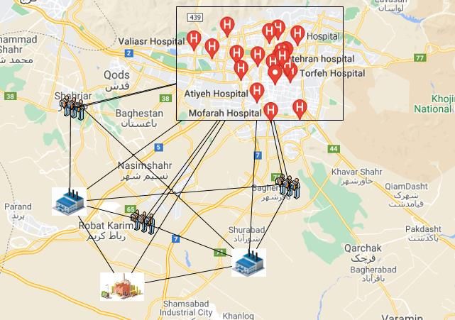
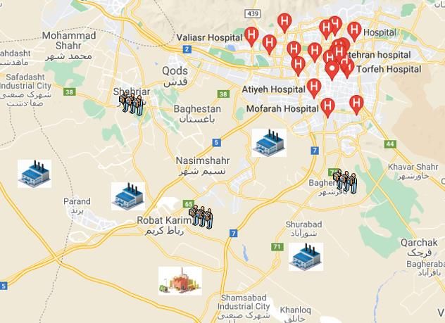
206 We show the potential location for assigning HC, WS, WPC, landfill in Tehran, Iran (cf. Figure
207 3). After solving the model, it suggests that we activate WS and determine the location and the
208 flow of VMWCND components. The objective function is 1520407 in Table 2 and the final
209 location-allocation is drawn in Figure 4. Finally, we calculate population risk (left-hand side of
210 Constraint (15)) that are 54026.33 persons. Eventually, we compare VMWCND with risk and
211 worst case and without risk and worst case in Table 5. We can see that by embedding risk and
212 worst case, the cost function is almost 1.65% greater than without risk and worst case.
Figure 3. Potential location for the facilities.
213
16214 Table 5. Comparing P1- VMWCND with risk and worst case and without risk and worst case.
P1- VMWCND
Model P1- VMWCND without risk and Gap
worst case
P1-main 1520407 1495346.97 1.65%
215
Figure 4. Final location for VMWCND facility.
216 4.1. Variation on the conservative coefficient
217 The conservative coefficient ( ) is the amount of conservative decision-makers. We change it by
218 varying between 0-1 that the conservation of decision-maker has been changed.
Figure 5. Cost function for different Lambda. Figure 6. Time solution for different Lambda.
17219 If the conservative coefficient increases to 1, the cost function grows in Table 6, Figure 5 and Figure 6. If
220 the conservative coefficient increases 50%, the cost function will increase by 1.65%, but time solution and
221 population risk do not change significantly.
222 Table 6. Effects of variation of conservative coefficient.
Conservative Cost Time Cost Population
Problem
coefficient ( ) function solution variation risk
P1 0.00 1495346.97 6.289 -1.65% 54026.33
P1 0.25 1507877.11 5.52 -0.82% 54026.33
P1-main model 0.5 1520407.25 9.422 0.00% 54026.33
P1 0.75 1532937.39 5.526 0.82% 54026.33
P1 1.00 1545467.53 6.4 1.65% 54026.33
223 4.2. Variation on confidence level of CVaR
224 The confidence level of CVaR ( ) is the amount of risk-averse decision-makers. If the confidence
225 level grows up, we can see, the cost function will increase (cf. Table 7 and Figure 7). By increasing
226 2% for confidence level, the cost function increase 0.03%.
227 Table 7. Effects of the confidence level of CVaR.
Time Cost
Problem Confidence level Cost function
solution variation
P1 1% 1519419.405 5.92 -0.06%
P1 2% 1519658.805 5.666 -0.05%
P1 3% 1519903.141 5.751 -0.03%
P1-main model 5% 1520407.25 5.45 0.00%
P1 6% 1520667.342 5.544 0.02%
P1 7% 1520933.032 5.728 0.03%
Figure 7. Effects of the confidence level of CVaR.
18228 4.3. Variation on waste recovery coefficient
229 The waste recovery coefficient ( ) is the ratio of waste that goes to landfills. If the waste recovery
230 coefficient grows, we can see that the cost function and population risk will decrease (cf. Figure
231 8, Figure 9 and Table 8). Increasing waste recovery coefficient, transportation to WPC increases
232 and then the cost function increase. But this issue helps systems to use and recover waste.
Figure 8. Effects of variation waste recovery Figure 9. Effects of variation waste recovery
coefficient on the cost function. coefficient on population risk.
233 Table 8. Effects of changing waste recovery coefficient.
Problem Waste recovery Cost Population
Cost function Time solution
coefficent variation risk
P1 30% 1523371 6.004 0.19% 54196
P1 25% 1522667 5.436 0.15% 54142.3
P1 15% 1521177 5.676 0.05% 54112.7
P1-main model 10% 1520407 5.45 0.00% 54026.3
P1 5% 1519622 5.967 -0.05% 53897.7
P1 0% 1518823 6.07 -0.10% 53662.3
234 4.4. Variation on demand
235 We test the effects of changing demand. By increasing demand, the cost function increase, too
236 (cf. Table 9). As can be seen, When the demand increases 40%, the cost function grows 12% and
237 when demand decreases 50%, it grows down 16% (cf. Figure 10 and Figure 11).
19Figure 10. Effects of variation demnad on cost Figure 11. Effects of variation demand on
function. population risk.
238 Table 9. Effects of changing demand.
Problem Changing Cost function Time Cost Population
demand solution variation risk
P1 -50% 1277474.078 5.941 -15.98% 53843.001
P1 -40% 1326060.712 5.888 -12.78% 53906.334
P1 -20% 1423233.979 6.528 -6.39% 53965.334
P1-main model 0% 1520407 5.45 0.00% 54026.334
P1 +20% 1617580.513 6.295 6.39% 54026.334
P1 +40% 1714753.780 5.963 12.78% 54026.334
239
240 4.5. Variation on scale of the main model
241 The several large-scale problems is defined in Table 10. When the scale of problems is increased,
242 the time solution and cost function increase in Figure 12 and Figure 13. As can be seen, the
243 proposed model show NP-hard and the behavior of this model is exponential for large scale.
244 Therefore, we need to solve the model by heuristic, metaheuristic and new exact solution in
245 minimum time on large scale.
246 Table 10. Cost and time solution for several problems.
Positive var.
Binary var.
Constraint
Free var.
Problem
i . j .c . k .t . s Cost Time Population
function solution risk
P1 118.4.3.1.3.3 4396 4393 12 8818 1520407 9.422 54026.33
P2 10.8.4.2.7.7 6280 6273 20 12380 609257 6.796 9201.68
20P3 118.4.3.1.3.5 7324 7321 16 14694 1591272 13.49 54408.4
P4 120.5.4.1.5.3 9380 9376 12 18721 1906117 21.548 91725.33
P5 120.5.4.2.7.3 13235 13231 12 36388 2160152 72.426 128016.7
P6 120.8.4.2.7.3 21176 21169 12 44578 2152882 249.904 127924
247
Figure 12. Cost function for several problems. Figure 13. Time solution for several problems.
248 5. Managerial insights and practical implications
249 We surveyed viable waste medical chain network design (VWMCND). We try to pay more
250 attention to five concepts in medical waste network design. We design VWMCND that considers
251 agility, resilience, sustainability, risks and robustness to cope with disruption and requirements of
252 government. As managers of the VWMCND, we should move forward to applying the novel
253 concept in MCND to decrease cost and population risk, increase the resiliency of facility,
254 robustness, risk-averse and agility of network. In this research, we have Health Center (HC), Waste
255 Segregation (WS), Waste Purchase Contractor (WPC) and landfill. We propose to locate WS to
256 decrease waste and recover them and send to the WPC. Recovering medical waste like metal and
257 plastic can help the environment and return to production cycle. In this situation of COVID-19 and
258 because of economic problem, we should use all power to utilize waste and move to circular
259 economy and sustainable development. This issue is compatible Sustainable Development Goal
260 (SDG12-Ensure sustainable consumption and production patterns) and the circular economy
261 pillars.
262 6. Conclusions and Outlook
263 Medical Waste Management (MWM) is an important and necessary problem in the COVID-19
264 situation for treatment staff. The number of infectious patients grows up and amount of MWMs
21265 increases day by day. We should think about this issue and find a solution for this issue. We suggest
266 to recovery MWM by waste segregation. Therefore, we proposed a novel Viable Medical Waste
267 Chain Network Design (VMWCND) that consider resiliency (flexibility and network complexity)
268 and sustainable (energy and environment) requirement. Finally, we try to tackle decrease risks and
269 increase robustness and agility to demand fluctuation and network. We utilize a novel two-stage
270 robust stochastic programming and solve with a GAMS CPLEX solver.
271 Therefore, the results are as follows:
272 1. If the conservative coefficient increases up to 1, the cost function grows up in If the
273 conservative coefficient increases to 1, the cost function grows in Table 6, Figure 5 and
274 Figure 6. If the conservative coefficient increases 50%, the cost function will increase by
275 1.65%, but time solution and population risk do not change significantly.
276 2. If the conservative coefficient increases up to 50%, the cost function will increase 1.65%,
277 but time solution and population risk do not change significantly.
278 3. If the confidence level of CVaR grows up, we can see, the cost function will increase (cf.
279 Figure 7 and Table 7). Increasing for confidence level by 2%, the cost function increase
280 0.03%.
281 4. If the waste recovery coefficient grows, we can see that the cost function and population
282 risk will decrease (cf. Figure 8, Figure 9 and Table 8). By increasing the waste recovery
283 coefficient, transportation to WPC increases and then the cost function increase. But it
284 helps systems to use waste and recover them.
285 5. When demand increases 40%, the cost function grows 12% and when demand decreases
286 50%, it grows down 16% (cf. Figure 10 and Figure 11).
287 6. When the scale of problems is increased, the cost function and time solution grow up in
288 Figure 12 and Figure 13. As can be seen, the behavior of the proposed model is NP-hard
289 and exponential on large scale. Therefore, we need to solve the model by heuristic,
290 metaheuristic and new exact solution in minimum time on large scale.
291 Finally, solving the main model on a large scale is the research constraint. We propose to apply
292 exact algorithms like benders decomposition, branch and price, branch and cut, column generation,
293 heuristic and meta-heuristic algorithms to solve models in minimum time (Fakhrzad & Lotfi, 2018;
22294 Lotfi, Mehrjerdi, & Mardani, 2017). We can add other resilience and sustainable tools to the model
295 until increasing the resiliency and sustainability of the model like backup facility and redundancy.
296 Further, we suggest adding coherent risk criteria like Entropic Value at Risk (EVaR) (Ahmadi-
297 Javid, 2012) for considering risks. Researchers intend to investigate method uncertainty like robust
298 convex (Lotfi, Mardani, & Weber, 2021). Using new and novel uncertainty methods like data-
299 driven robust optimization is advantageous for a conservative decision-maker in the recent decade.
300 Eventually, we suggest equipping VMWCND with novel technology like blockchain for the
301 viability of MWCND.
302 7. Ethical Approval
303 Not applicable
304 8. Consent to Participate
305 Not applicable
306 9. Consent to Publish
307 Not applicable
308 10. Authors Contributions
309 Reza Lotfi: conceptualization, supervision, software, methodology; software; formal analysis;
310 data curation; writing original draft; visualization;
311 Bahareh Kargar: methodology; software; formal analysis; data curation; writing original draft;
312 writing review and edit; visualization;
313 Alireza Gharehbaghi: methodology, validation;
314 Gerhard-Wilhelm Weber: validation, writing review and edit;
315 11. Funding
316 There is not funding.
317 12. Competing Interests
318 The authors declare no competing interests.
319 13. Availability of data and materials
320 Not applicable
321 References
322 Ahmadi-Javid, A. (2012). Entropic value-at-risk: A new coherent risk measure. Journal of Optimization Theory and
323 Applications, 155(3), 1105-1123.
324 Aung, T. S., Luan, S., & Xu, Q. (2019). Application of multi-criteria-decision approach for the analysis of medical
325 waste management systems in Myanmar. Journal of Cleaner Production, 222, 733-745.
23326 Budak, A., & Ustundag, A. (2017). Reverse logistics optimisation for waste collection and disposal in health
327 institutions: the case of Turkey. International Journal of Logistics Research and Applications, 20(4), 322-
328 341.
329 Fakhrzad, M.-B., & Lotfi, R. (2018). Green vendor managed inventory with backorder in two echelon supply chain
330 with epsilon-constraint and NSGA-II approach. Journal of Industrial Engineering Research in Production
331 Systems, 5(11), 193-209.
332 Goli, A., Zare, H. K., Tavakkoli-Moghaddam, R., & Sadeghieh, A. (2019). Application of robust optimization for a
333 product portfolio problem using an invasive weed optimization algorithm. Numerical Algebra, Control &
334 Optimization, 9(2), 187-209.
335 Gondal, I. A., & Sahir, M. H. (2013). Model for biomass‐based renewable hydrogen supply chain. International
336 Journal of Energy Research, 37(10), 1151-1159.
337 Homayouni, Z., & Pishvaee, M. S. (2020). A bi-objective robust optimization model for hazardous hospital waste
338 collection and disposal network design problem. Journal of Material Cycles and Waste Management, 22(6),
339 1965-1984.
340 Ivanov, D. (2020). Viable supply chain model: integrating agility, resilience and sustainability perspectives—lessons
341 from and thinking beyond the COVID-19 pandemic. Annals of Operations Research, 1-21.
342 Ivanov, D., & Dolgui, A. (2020). Viability of intertwined supply networks: extending the supply chain resilience
343 angles towards survivability. A position paper motivated by COVID-19 outbreak. International Journal of
344 Production Research, 58(10), 2904-2915.
345 Kara, G., Özmen, A., & Weber, G.-W. (2019). Stability advances in robust portfolio optimization under parallelepiped
346 uncertainty. Central European Journal of Operations Research, 27(1), 241-261.
347 Kargar, S., Paydar, M. M., & Safaei, A. S. (2020). A reverse supply chain for medical waste: A case study in Babol
348 healthcare sector. Waste Management, 113, 197-209.
349 Kargar, S., Pourmehdi, M., & Paydar, M. M. (2020). Reverse logistics network design for medical waste management
350 in the epidemic outbreak of the novel coronavirus (COVID-19). Science of the Total Environment, 746,
351 141183.
352 Li, H., Hu, Y., Lyu, J., Quan, H., Xu, X., & Li, C. (2021). Transportation Risk Control of Waste Disposal in the
353 Healthcare System with Two-Echelon Waste Collection Network. Mathematical Problems in Engineering,
354 2021.
355 Lotfi, R., Mardani, N., & Weber, G. W. (2021). Robust bi‐level programming for renewable energy location.
356 International Journal of Energy Research.
357 Lotfi, R., Mehrjerdi, Y. Z., & Mardani, N. (2017). A multi-objective and multi-product advertising billboard location
358 model with attraction factor mathematical modeling and solutions. International Journal of Applied Logistics
359 (IJAL), 7(1), 64-86.
360 Lotfi, R., Mehrjerdi, Y. Z., Pishvaee, M. S., Sadeghieh, A., & Weber, G.-W. (2021). A robust optimization model for
361 sustainable and resilient closed-loop supply chain network design considering conditional value at risk.
362 Numerical Algebra, Control & Optimization, 11(2), 221.
363 Mantzaras, G., & Voudrias, E. A. (2017). An optimization model for collection, haul, transfer, treatment and disposal
364 of infectious medical waste: Application to a Greek region. Waste Management, 69, 518-534.
365 Narayanamoorthy, S., Annapoorani, V., Kang, D., Baleanu, D., Jeon, J., Kureethara, J. V., & Ramya, L. (2020). A
366 novel assessment of bio-medical waste disposal methods using integrating weighting approach and hesitant
367 fuzzy MOOSRA. Journal of Cleaner Production, 275, 122587.
368 Nikzamir, M., Baradaran, V., & Panahi, Y. (2021). A Supply Chain Network Design for Managing Hospital Solid
369 Waste. Journal of Industrial Management Studies, 19(60), 85-120.
370 Saeidi-Mobarakeh, Z., Tavakkoli-Moghaddam, R., Navabakhsh, M., & Amoozad-Khalili, H. (2020). A bi-level and
371 robust optimization-based framework for a hazardous waste management problem: A real-world application.
372 Journal of Cleaner Production, 252, 119830.
373 Saeidi-Mobarakeh, Z., Tavakkoli-Moghaddam, R., Navabakhsh, M., & Amoozad-Khalili, H. (2020). A Bi-level Meta-
374 heuristic Approach for a Hazardous Waste Management Problem. International Journal of Engineering,
375 33(7), 1304-1310.
376 Sepúlveda, J., Banguera, L., Fuertes, G., Carrasco, R., & Vargas, M. (2017). Reverse and inverse logistic models for
377 solid waste management. South African Journal of Industrial Engineering, 28(4), 120-132.
378 Shadkam, E. (2021). Cuckoo optimization algorithm in reverse logistics: A network design for COVID-19 waste
379 management. Waste Management & Research, 0734242X211003947.
380 Sherali, H. D., & Adams, W. P. (2013). A reformulation-linearization technique for solving discrete and continuous
381 nonconvex problems (Vol. 31): Springer Science & Business Media.
24382 Soleimani, H., & Govindan, K. (2014). Reverse logistics network design and planning utilizing conditional value at
383 risk. European journal of operational research, 237(2), 487-497.
384 Suksee, S., & Sindhuchao, S. (2021). GRASP with ALNS for solving the location routing problem of infectious waste
385 collection in the Northeast of Thailand. International Journal of Industrial Engineering Computations, 12(3),
386 305-320.
387 Tirkolaee, E. B., Abbasian, P., & Weber, G.-W. (2021). Sustainable fuzzy multi-trip location-routing problem for
388 medical waste management during the COVID-19 outbreak. Science of the Total Environment, 756, 143607.
389 Tirkolaee, E. B., & Aydın, N. S. (2021). A sustainable medical waste collection and transportation model for
390 pandemics. Waste Management & Research, 0734242X211000437.
391 Tsai, W.-T. (2021). Analysis of medical waste management and impact analysis of COVID-19 on its generation in
392 Taiwan. Waste Management & Research, 0734242X21996803.
393 Wang, Z., Huang, L., & He, C. X. (2019). A multi-objective and multi-period optimization model for urban healthcare
394 waste’s reverse logistics network design. Journal of Combinatorial Optimization, 1-28.
395 Yu, H., Sun, X., Solvang, W. D., Laporte, G., & Lee, C. K. M. (2020). A stochastic network design problem for
396 hazardous waste management. Journal of Cleaner Production, 277, 123566.
397 Yu, H., Sun, X., Solvang, W. D., & Zhao, X. (2020). Reverse logistics network design for effective management of
398 medical waste in epidemic outbreaks: Insights from the coronavirus disease 2019 (COVID-19) outbreak in
399 Wuhan (China). International journal of environmental research and public health, 17(5), 1770.
400
25You can also read