Machine Learning for Professional Tennis Match Prediction and Betting - CS229
←
→
Page content transcription
If your browser does not render page correctly, please read the page content below
Machine Learning for Professional Tennis Match Prediction and Betting

                                  Andre Cornman, Grant Spellman, Daniel Wright

                         Abstract                                    1.3. Related Work
                                                                         There are a number of papers related specifically to mod-
    Our project had two main objectives. First, we wanted
                                                                     eling and machine learning techniques for tennis betting.
to use historical tennis match data to predict the outcomes
                                                                     Barnett uses past match data to predict the probability of a
of future tennis matches. Next, we wanted to use the predic-
                                                                     player winning a single point [4]. This prediction is then ex-
tions from our resulting model to beat the current betting
                                                                     tended to predict the probability of winning a match. Their
odds. After setting up our prediction and betting models,
                                                                     approach claims a 6.8% return on investment for the 2011
we were able to accurately predict the outcome of 69.6% of
                                                                     WTA Grand Slams. Clarke and Dyte used a logistic regres-
the 2016 and 2017 tennis season, and turn a 3.3% profit per
                                                                     sion to predict match outcomes by using the difference in
match.
                                                                     the ATP rankings of players [5]. Both of these models used
                                                                     a single feature to predict outcome. However, Somboon-
                                                                     phokkaphan used artificial neural network (ANN) using a
1. Introduction                                                      number of features (including previous match outcomes,
                                                                     first serve percentage, etc.) [6]. This model had a 75% ac-
1.1. Motivation                                                      curacy for predicting matches in the 2007 and 2008 Grand
                                                                     Slam tournaments.
    Tennis is an international sport, enjoyed by fans in coun-
tries all over the world. Unsurprisingly, professional tennis
players come from an equally diverse background, drawn               2. Datasets
from countries throughout North America, South America,
Europe and Asia. From each of these regions players come                 Tennis match data was retrieved from an open source
equipped with different playing styles and specialties. In           data set available on GitHub [1]. It includes all match re-
addition to this, tennis fans know that the sport is played          sults from the Open Era (1968) to September of this year.
on three unique surfaces (clay, grass, and hard courts), each        More recent matches (after the year 2000) include match
lending itself to different play strategies. There are a huge        statistics such as the number of aces hit, break points faced,
number of variables that define each and every tennis match,         number of double faults, and more. Betting data was re-
making the sport both exciting and unpredictable. Being              trieved from [2], which has odds from various betting ser-
tennis fans ourselves, we decided to move away from our              vices from 2001 on. The data here also includes match
gut instincts and take a new approach to predicting the out-         scores. Ultimately, these two datasets had to be merged so
comes of our favorite matches.                                       that we could incorporate the betting odds into our predic-
                                                                     tion model along with the match results and statistics. We
                                                                     were able to merge about 93% of the data. The merged
1.2. Project Outline
                                                                     dataset has 46,114 matches. This was split into a training
    The data from our project came primarily from author             set of size 41,324 and a test set of 4,790 (roughly a 90-10
and sports data aggregator Jeff Sackmann [1], as well as             split).
betting data from Tennis-Data.co.uk [2]. See the dataset                 In the data, the statistics, odds, etc., were labeled only
section for more details. Once we combined and processed             for the winner and loser, so for each match we randomly
this data, we tried fitting it to different models to see see        assigned “Player 1” to be either the winner or loser, and
which prediction model yielded the best performance for              “Player 2” to be the other person. We also added a la-
predicting match outcomes. The classification models we              bel for each match as to whether Player 1 won the match.
tried include logistic regression, SVM, random forests and           This would be the label that our model would try to predict.
neural networks. Finally, we incorporated our prediction             These random labellings were done once as part of our data
model into a single shot decision problem to decide, for a           pre-processing and then were held constant through the rest
given match, who to bet on, or whether to bet all.                   of the project.

                                                                 1
2.1. Feature Engineering and Selection 3.2. SVM
The merged data set offered a large number of poten- While fitting our data to an SVM model, we tried a num-
tial features that we could use to train our model, includ- ber of kernels with varying results. In general, a SVM
ing player rankings, ranking points, age, height, as well as model solves the problem for a data set (x(i) , y (i) ) where
in-match statistics including aces, break points and double i = 1, 2, ...m, given by
faults.
||w||2
In addition to these features, we also computed a num- minγ,w,b 2 s.t. γ (i) ≥ 1 for all i = 1, 2, ...m
ber of our own features to capture a player’s recent perfor-
mance. For each match, we calculated the average of each where the geometric margin γ (i) is equal to
match statistic over the most recent 5, 10, and 20 matches. w T (i) b
γ (i) = y (i) (( ||w|| ) x + ||w|| )
Finally, we calculated a players head to head record against
their opponent, both overall and with respect to the given The specifications for the SVM problem shown here are
play surface. Altogether, we hoped that these additional given by Stanford CS229 lecture notes, and further details
features could help quantify the current state of a player’s and intuition for the SVM problem can be found there [7].
game.
All features were of the following form: 3.3. Neural Network
FEATUREi = STATi,player1 − STATi,player2 A neural network is composed of “layers.” The input
to each layer is either the data itself or the output from a
This means the features we trained on were all differ- previous layer. Each layer applies a linear transformation to
ences between certain statistics about the players (such as the data and then an activation function, which is typically
ranking, ranking points, head-to-head wins, etc.). This was nonlinear. Mathematically, this is represented as:
done to achieve symmetry. We wanted a model where the
labeling of the players as Player 1 or Player 2 doesn’t mat- z [i] = W [i] a[i−1] + b[i]
ter. This would help us to avoid any inherent bias to/for the a[i] = g(z [i] )
player randomly labeled as “Player 1” [3].
Here a[i] represents the output vector for each layer and
3. Methods g is the activation function. The output of the last layer is
We decided to try a number of machine learning algo- the output of the network. The input to the first layer a[0] is
rithms. We briefly summarize how each works below. the original data, x.
The neural network needs to learn the weight arrays,
3.1. Logistic Regression W [i] and biases, b[i] . This can be done by “back-
In logistic regression, we have a hypothesis of the form: propagation” which uses gradient descent (typically batch
gradient descent) to update the parameters until conver-
1 gence. In batch gradient descent, rather than using just a
hθ (x) = g(θT x) = ,
1 + e−θT x single example (stochastic gradient descent) or the entire
dataset to calculate the gradient of the parameters, the gra-
where g is the logistic function. We assume that the binary
dient is computed for “batches” of data. The batch size of
classification labels are drawn from a distribution such that:
the gradient descent is a hyperparameter of the algorithm.
P (y = 1 | x; θ) = hθ (x)
3.4. Random Forest
P (y = 0 | x; θ) = 1 − hθ (x)
A random forest model is a nonparametric supervised
Given a set of labeled set of training examples, we learning model. It is a generalization of a random tree
choose θ to maximize the log-likelihood: model in which several decision trees are trained.
X A tree is grown by continually “splitting” the data (at
`(θ) = y (i) log h(x(i) ) + (1 − y (i) ) log(1 − h(x(i) )) each node of the tree) according to a randomly chosen sub-
i set of the features. The split is chosen as the best split for
We can maximize the log-likelihood by stochastic gra- those features (meaning it does the best at separating posi-
dient ascent under which the update rule is the following tive from negative examples).
(where α is the learning rate) and we run until the update is A random forest is made up of many trees (how many is
smaller than a certain threshold: a hyperparameter of the model) trained like this. Given a
data point, the output of a random forest is the average of
θ ← θ + α(y (i) − hθ (x(i) )x(i) the outputs of each tree for that data point.
24. Experimental Results for a d degree expansion of the features. We tried a
second degree polynomial fit. Similar to the RBF ker-
We first discuss the results for the machine learning clas- nel, the polynomial kernel was very slow to train and
sification algorithms we tried. prone to over fitting. This is likely due to our large fea-
ture space, where the polynomial kernel would create
a larger number of higher order term and cross term
Model Train 5-Fold CV
features.
Random Forest 73.5 69.7
Neural Network 81.8 65.2
(1 HL, 300 nodes, logit.)
SVM
→ Linear Kernel 69.8 69.9
→ RBF Kernel 51.0
→ Polynomial Degree 3 54.0*
Logistic Regression w/L1 Reg. 69.9 3. Linear: The linear term only uses a linear weighting
Logistic Regression w/L2 Reg 69.7 of the first order of the feature set. The linear kernel
Table 1. Training and 5-Fold Cross Validation Accuracies for proved to be the most appropriate for our data. It was
Models faster to train and allowed us to more finely tune the
*SVM with polynomial kernel was too slow to validate hyper-parameters, further increasing prediction accu-
racy. In addition to this, we were able to experiment
with the ensemble library in sklearn to better estimate
the linear parameters. Ultimately, this kernel gave us
4.1. Logistic Regression
the best performance under the SVM model.
Logistic regression had good accuracy in 5 fold cross
validation, however training the model was very slow to
run. We were able to perform tuning of the regularization
strength for L1 and L2 regularization, which both resulted
in low variance. We think that adding polynomial terms
might help, but we did not have the computational resources 4.3. Random Forests
to be able to carry out these experiments in a reasonable
timeframe.
The random forest model had the advantage of being
4.2. SVM much faster to train. This allowed us to more easily iter-
We tried three different SVM kernels for our model: ate with the model. For example, it was easier to tune the
RBF, polynomial, and linear. A general discussion of each hyperparameters because training the model several times
follows below. For the respective training model accuracies, for cross validation was not too computationally expensive.
see Table 1.
1. RBF: Also known as the Gaussian kernel, the feature One of the hyperparamters we tuned was the minimum
mapping is of the form samples per leaf. When this was set to one, i.e., the leafs
could be as small as a single match, the training accuracy
||x−z||22 was 100% while the cross-validation accuracy was only
K(x, z) = exp(− 2σ 2 ) around 69%. This represents poor generalization and ex-
treme overfitting to the training set. We tuned this param-
From the form of the kernel, we can see that it gives an eter to be 50, which reduced the training accuracy to 73%
estimate of roughly how far apart x and z are. When and increased the cross-validation accuracy modestly, im-
trying this kernel, the model was slow to train and proving generalization.
prone to over fitting, even as we tried various hyper-
parameters like the regularization strength. Because of
the size of our training set, and the non-linear nature of Below is the calibration curve for the random for-
the kernel, this model proved to be impractical. est model. For 10 “buckets” it plots the mean pre-
dicted value against the fraction of “positives,” which in
2. Polynomial: The polynomial kernel has the form of this case means player 1 winning. The curve shows
that the random forest model is extremely well cal-
K(x, z) = (xT z)d ibrated. This is important for our betting strategy.
3matches, and, interestingly age.
4.4. Neural Network
We thought that a neural network might be useful in dis-
covering non-linearities. However, the accuracy of the neu-
ral network was not as high as the other models. It is possi-
ble that this would have improved if we continued to try to
tune the hyperparameters of the model (such as the number
of hidden layers, the nodes per hidden layers, the activation
function, etc.) but the time it took to train was prohibitive
to do on our own computers.
5. Betting Model Results
We developed a simple betting model that uses the out-
put of our random forest model and the odds data to bet on
One can extract “feature importances” from a random the player that maximizes the expected returns. The odds
forest model. These are computed as the mean decrease in data is represented as two numbers per match (greater than
node “impurity” for that feature across all trees, where node 1). For example, if you bet correctly on player 1, who’s
impurity is a measure of how separated the data is (by posi- odds are 1.5, then for each dollar you bet, you win 0.5 dol-
tive/negative label). Below are the estimated feature impor- lars. However, if you bet incorrectly, you lose the initial bet
tances from our trained random forest model. amount.
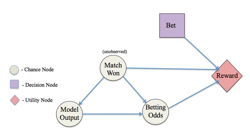
Figure 2. Decision network for single-shot betting strategy.
We modeled our betting strategy as a single-shot deci-
sion problem for each match, where we aim to maximize
the expected earnings. This was a better approach than, say,
a reinforcement learning approach because there is no sense
of underlying system dynamics in this setting: that is, there
is no real reason for one match to “transition” to another.
Instead, each match should be thought of as an independent
decision problem.
Figure 1. 10 most important features in the random forest model. Possible actions include betting 1 dollar on player 1, bet-
The black lines indicate the standard deviation of the importance ting 1 dollar on player 2, and not betting. The strategy
estimate (estimated as the standard deviation of the feature impor- chooses the action with the highest expected reward:
tance across trees). The feature importances are normalized to sum
to one over all features.
b∗ = arg max E[U (win, odds, b)]
b∈{0,+1,−1}
The first five of these features refer to betting data:
“Max” refers to the best betting odds, “Avg” refers to the On test set data, the betting strategy earns an average of
average betting odds across all quoted odds, and “B365”, 3.3% per match. Interestingly, the strategy takes the no bet
“EX,” and “PS” refer to the odds of specific betting ser- action 29% of the time, where the expected utility of betting
vices. The most important non-betting related features are on either player is negative. We also find it interesting that
the difference in rank, ranking points, wins in the last 20 the betting strategy has streaks of winning, and streaks of
4This aspect of the model could potentially be improved
by a dataset with richer features, such as injury informa-
tion about each player, more fine-grained statistics, weather,
coaching, strategy, etc.
7. Future Work
First and foremost, we are excited to try out our predic-
tion model on upcoming tournaments in the 2018 season.
Perhaps we can give ourselves an edge on the betting web-
sites.
As for our prediction model, it would be very interest-
ing to further explore and properly validate the models that
demanded more computational power than we had avail-
able to do our project. This would be relevant primarily for
Figure 3. Cumulative winnings on the test set for simple betting
the non-linear SVM models, logistic regression model, and
strategy.
neural network model. Because of the size of our dataset
(approximately 45,000 rows with upwards of 80 features),
losing, however we do not have a good explanation for this it was difficult to train and tune these models locally on our
result. machines. In particular, we were able to train these models
We computed the Sharpe ratio for our strategy over this on our dataset, however, the difficulty came in when iterat-
period. The Sharpe ratio is a commonly used evaluation ing over the hyper-parameters of these models. Given more
metric for strategies in financial markets and is defined as computational resources, we could optimize these hyper-
the mean return over the standard deviation of the returns. parameters. With regards to our betting model, one goal of
The Sharpe ratio for our strategy was 0.02, which would be ours is to add more flexibility to our betting decision model.
considered very poor in the financial industry. We think that For instance, our current model only makes $1 bets, or no
this can be explained by the substantial risk of losing all of bets at all. It would be interesting to scale our bets to larger
one’s money in a given bet, which causes the standard devi- or smaller amounts given the confidence reported by our
ation for the return across all bets to be quite high. People model. For example, we could adjust the bet amount based
who gamble on sports, one might hypothesize, are attracted on the difference between the model output probability and
to risk, rather than averse to it. the odds data probability of a player winning.
6. Error Analysis 8. Contributions
Below are tables, similar to confusion matrices, for our 8.1. Andre
random forest model on the test set. We see that most of
I worked on setting up and implementing the betting
the time, the model is predicting the higher ranked player
strategy.
and the favored player. (Here favored means the player has
more favorable odds.) In fact, on the test set, the model is 8.2. Danny
predicting worse than 50% when it predicts the disfavored
player. I worked on merging the two datasets and on feature en-
gineering and building/testing models (logistic regression,
Predicted Total # Correct Pct. neural network, random forest).
Lower Ranked Player 814 486 59.7 8.3. Grant
Higher Ranked Player 3976 2850 71.7
I worked on setting up and testing all of the SVM models
Predicted Total # Correct Pct. we tried to fit to our merged data set. I cross validated these
Favored Player 4669 3279 70.2 models as well.
Disfavored Player 121 57 47.1
References
This indicates that our model is not capturing insights [1] https://github.com/JeffSackmann/tennis atp , Jeff Sack-
about when/why a lower-ranked or disfavored player would mann
win a match (and instead mostly relies on these features for
its predictiveness). [2] http://www.tennis-data.co.uk/alldata.php
5[3] https://www.doc.ic.ac.uk/teaching/distinguished-
projects/2015/m.sipko.pdf , Section 3.1.2 Michal Sipko
and Dr. William Knottenbelt of the Imperial College
London
[4] T. Barnett and S. R. Clarke. Combining player statistics
to predict outcomes of tennis matches. IMA Journal of
Management Mathematics, 16:113120, 2005.
[5] S. R. Clarke and D. Dyte. Using official ratings to sim-
ulate major tennis tournaments. International Transac-
tions in Operational Research, 7(6):585594, 2000.
[6] A. Somboonphokkaphan, S. Phimoltares, and C.
Lursinsap. Tennis Winner Prediction based on Time-
Series History with Neural Modeling.IMECS 2009: In-
ternational Multi-Conference of Engineers and Com-
puter Scientists, Vols I and II, I:127132, 2009.
[7] http://cs229.stanford.edu/notes/cs229-notes3.pdf ,
Stanford University, CS229 Lecture Notes, Andrew Ng
6You can also read