Development and validation of prediction models Statistics in Practice II - Biometrische Gesellschaft

Development and validation of
 prediction models

 Statistics in Practice II

 Ben Van Calster
 Department of Development and Regeneration, KU Leuven (B)
 Department of Biomedical Data Sciences, LUMC (NL)
 Epi-Centre, KU Leuven (B)

Biometrisches Kolloquium, 16th of March 2021

1. Model performance and validation
(focus on binary outcomes)

Model validation is important!

Altman & Royston, Stat Med 2000. Altman et al, BMJ 2009.
Steyerberg et al, Epidemiology 2010. Koenig et al, Stat Med 2007. 3

Model validation?

It is not primarily about statistical significance of

1. The predictors

2. A goodness-of-fit test like the Hosmer-Lemeshow test or its variants

Although: a GOF test does give a gist of what is important
 agreement between predictions and observations
 CALIBRATION

 4

Calibration is complicated

 5

Calibration is complicated

 6

Level 1: Mean calibration

Mean estimated risk = observed proportion of event

“On average, risks are not over- or underestimated.”

O:E ratio: observed events / expected events

If violated: adjust intercept.

 7

Level 2: Weak calibration

Mean AND variability/spread of estimated risk is fine

“On average, risks are not over- or underestimated, nor too extreme/modest.”

Logistic calibration model: = + ∗ 
 1− 

Calculate - calibration slope: (cf spread) → should be 1
 - calibration intercept: | =1 (cf mean) → should be 0

If violated: adjust intercept and coefficients using + ∗ 

 8

Level 3: Moderate calibration

Estimated risks are correct, conditional on estimated risk.

“Among patients with estimated risk , the proportion of events is .”

Flexible calibration model: = + 
 1− 

Calibration curve.

If violated: refit model, perhaps re-evaluate functional form.

 9

Level 4: Strong calibration

 Estimated risks are correct, conditional on covariate pattern.

 “Per covariate pattern, the proportion of events equals the estimated risk.”

 In short, the model is fully correct.

Vach W. Regression models as a tool in medical research. Boca Raton: Chapman and Hall/CRC; 2013. 10

Miscalibration Mean

 Weak Moderate

 Strong

Van Calster and Steyerberg. Wiley StatsRef 2018. https://doi.org/10.1002/9781118445112.stat08078. 11

Calibration assessment

Van Calster et al. J Clin Epidemiol 2016;74:167-176. 12

Discrimination

Calibration: ~ absolute performance
Discrimination: ~ relative performance

Do I estimate higher risks for patients with vs without an event?

C-statistic, equal to AUROC for binary outcomes.

 13

Discrimination
 C or AUROC is interesting, ROC not so much.

 ROC shows classification results but ‘integrated over’ threshold. But
 classification critically depends on threshold! ROC = bizarre.

 (Pun intended.)

Verbakel et al. J Clin Epidemiol 2020;126:207-216. 14

15

Discrimination
 If you want a plot...

Karandeep Singh. Runway r package. https://github.com/ML4LHS/runway. 16

Overall measures

E.g. Brier score, R-squared measures (including IDI).

For model validation, I prefer to keep discrimination and calibration
separate.

 17

Statistical validity = clinical utility?

Discrimination and calibration: how valid is the model?

That is not the full story. In the end, clinical prediction models are made to
support clinical decisions!

To make decisions about giving ‘treatment’ or not based on the model, you
have to classify patients as high and low risk.

Classifications can be right or wrong: the classical 2x2 table

 EVENT NO EVENT

 HIGH RISK True Positive False positive

 LOW RISK False Negative True negative

 18

Clinical utility

 A risk threshold is needed. Which one?

 Myth! The statistician can calculate the threshold from the data.
 Myth! A threshold is part of the model.
 → “Model BLABLA has sensitivity of 80%” makes little sense to me.

Wynants et al. BMC Medicine 2019;17:192. 19

Clinical utility

ISSUE 1 – A RISK THRESHOLD HAS A CLINICAL MEANING

What are the utilities (U) of TP, FP, TN, FN?

 1 1 
Then threshold = − = =
 1+ 1+ + 
 − 

Hard to determine.
Instead of fixing U values, start with T: at which threshold are you uncertain
about ‘treatment’?

 20

Clinical utility

You might say: I would give ‘treatment’ if risk >20%, not if

Clinical utility

 Net Benefit (Vickers & Elkin 2006), even Charles Sanders Peirce (1884)

 When you classify patients, TPs are good and FPs are bad
 Net result: good stuff minus bad stuff: − .

 But: relative importance of TP and FP depends on T!
 o If T=0.5, = ; else < or >.
 o Harm of FP is odds(T) times the Benefit of a TP

 − ∗ 
 =
 
Vickers & Elkin. Med Decis Making 2006;26:565-574.
Peirce. Science 1884;4:453-454.
 22

Clinical utility

 ISSUE 2 – THERE IS NO SINGLE CORRECT THRESHOLD

 Preferences and settings differ, so Harm:Benefit and T differ.

 Specify a ‘reasonable range’ for T.

 Calculate NB for this range, and plot results in a decision curve
 → Decision Curve Analysis

Vickers et al. BMJ 2016;352:i6.
Van Calster et al. Eur Urol 2018;74:796-804.
Vickers et al. Diagnostic and Prognostic Research 2019;3:18. 23

Clinical utility

DCA is a simple research method. You don’t need anything special. It is useful to
assess whether a model can improve clinical decision making. It does not replace a
cost-effectiveness analysis, but can inform on further steps.

 24

Clinical utility

 ISSUE 3 – CPM ONLY ESTIMATES WHETHER RISK>T OR NOT

 T is independent of any model.

 If the model is miscalibrated, you may select too many (risk overestimated)
 or too few (risk underestimated) patients for treatment!

 Miscalibration reduces clinical utility, and may make the model worse than
 treating all/none! (Van Calster & Vickers 2015)

 NB nicely punishes for miscalibration.

Van Calster & Vickers. Medical Decision Making 2015;35:162-169. 25

Clinical utility

Models can be miscalibrated!
 → So pick any threshold with a nice combination of sensitivity and
 specificity!

That does not solve the problem in my opinion.

You may need a different threshold in a new hospital.

So you may just as well recalibrate the model.

 26

Types of validation: evidence pyramid…
(I love evidence pyramids)

 Different dataset
 EX- Hence: different population
 TERNAL
 Same dataset
 Hence: same population
 INTERNAL
 Exact same data
 No real validation
 APPARENT Optimistic

 27

Only apparent validation?

 Criminal behavior!

https://lacapitale.sudinfo.be/188875/article/2018-02-08/arrestation-braine-lalleud-dun-cambrioleur-recherche 28

Internal validation

• Only assessment of overfitting: c-statistic and slope sufficient.
• Skepticism: who will publish a paper with poor internal validation?
• Which approach?

 29

Internal validation

 • Train – test split
 o Inefficient: we split up the data into smaller parts
 o “Split sample approaches only work when not needed” (Steyerberg & Harrell 2016)
 o But: it evaluates the fitted MODEL!

 • Resampling is preferred
 o Enhanced bootstrap (statistics) or CV (ML) recommended
 o Efficient: you can use all data to develop the model
 o But: it evaluates the modeling PROCEDURE! (Dietterich 1998)
 o It evaluates expected overfitting from the procedure.

Steyerberg & Harrell. Journal of Clinical Epidemiology 2016;69:245-247.
Dietterich. Neural Computation 1998;10:1895-1923. 30

Calibration slope based on bootstrapping
 • Negative correlation with true slope, variability underestimated
 • Example (Van Calster 2020)
 o 5 predictors, development N=500, 10% event rate, 1000 repetitions
 o Every repetition: slope estimated using bootstrapping
 o Estimated slope: median 0.91, IQR 0.89-0.92, range 0.78-0.96
 o True slope: median 0.88, IQR 0.78-0.99, range 0.53-1.53
 o Spearman rho -0.72

Van Calster et al. Statistical Methods in Medical Research 2020;29:3166-3178. 31

External validation
 • Results affected by overfitting and by differences in setting (case-mix,
 procedures, …)
 • The real test: including ‘an external validation’ settles the issue, right?

Nevin & PLoS Med Editors. PLoS Medicine 2018;15:e1002708. 32

2. Expect heterogeneity

Expect heterogeneity

 • Between settings: case-mix, definitions and procedures, etc…

Luijken et al. J Clin Epidemiol 2020;119:7-18. 34

Expect heterogeneity

 • Across time: population drift (Davis et al, 2017)

Davis et al. Journal of the American Medical Informatics Association 2017;24:1052-1061. 35

THERE IS NO SUCH THING AS A VALIDATED MODEL

Validation is important!

But it’s complicated
 o Internal and external validations added to model development study
 may be tampered with (cynical take)
 o Internal validation has limitations

 o An external validation (whether good or bad) in one setting does not
 settle the issue
 o Performance tomorrow may not be the same as yesterday

So: assess/address/monitor heterogeneity

 36

Address heterogeneity
• Multicenter studies

• IPD

 37

Address heterogeneity

Debray et al. Statistics in Medicine 2013;32:3158-3180. 38

Development: random effects models
Address heterogeneity in baseline risk using random cluster intercepts

 = + + ,
 1− 
with ~ 0, 2 .

Heterogeneity in predictor effects can be assessed with random slopes

 = + + 1 1 + 1, + 2 2 + 2, ,
 1− 
 2 , , 2
 0
 2
with 1, ~ 0 , , 1 , 
 2, 0 , 2 1, 2 2
 2

 39

Development: fixed cluster-level effects

Add fixed parameters to model that describe the cluster

E.g. type of hospital, country

Can be done in combination with random effects

 40

Development: Internal-external CV
 k-fold CV IECV

 Leuven Leuven

 London London

 Berlin Berlin

 Rome Rome

Royston et al. Statistics in Medicine 2004;23:906-926.
Debray et al. Statistics in Medicine 2013;32:3158-3180.
 41

Model validation in clustered data

Riley et al. BMJ 2016;353:i3140.
Debray et al. Statistical Methods in Medical Research 2019;28:2768-2786.
 42

Model validation in clustered data

 1. Obtain cluster-specific performance
 2. Perform random-effects meta-analysis (Snell 2018, Debray 2019)

 c statistic: ~ , + 2

 O:E ratio: ~ , + 2

 Calibration intercept: ~ , + 2

 Calibration slope: ~ , + 2

Snell et al. Statistical Methods in Medical Research 2018;28:3505-3522.
Debray et al. Statistical Methods in Medical Research 2019;28:2768-2786.
 43

Model validation in clustered data

 One-stage model for calibration slopes:

 =1
 = + + ∗ + ∗ , where
 1− =1

 0 2 
 ~ , .
 0 2

 is overall calibration slope.
 are used to estimate center-specific slopes.

 (Bouwmeester 2013; Wynants 2018)

Bouwmeester et al. BMC Medical Research Methodology 2013;13:19.
Wynants et al. Statistical Methods in Medical Research 2018;27:1723-1736.
 44

Model validation in clustered data

• For calibration intercepts, the slopes are set to 1:

 =1
 = ′ + ′ + , where
 1− =1

 ′ ~ 0, 2′ .

 ′ is overall calibration intercept.
 ′ are used to estimate center-specific intercepts.

 45

Model validation in clustered data

 • Net Benefit at several reasonable thresholds (Wynants 2018):

 Bayesian trivariate random-effects MA of prevalence, sensitivity, specificity.

 1 12 12 1 2 13 1 3
 ~ 2 , 12 1 2 22 23 2 3
 3 13 1 3 23 2 3 32
 
 Optimal specification of (vague) priors: after reparameterization
 - Vague normal priors for 
 - Weak Fisher priors for correlations
 - Weak half-normal priors for variances

Wynants et al. Statistics in Medicine 2018;37:2034-2052. 46

Meta-regression & subgroup analysis

 • Largely exploratory undertaking, unless many big clusters

 • Meta-regression: add cluster-level predictors to meta-analysis
 o Mean, SD or prevalence of predictors per cluster
 o Can also be added to one-stage calibration analysis

 • Subgroup analysis?
 o Conduct the meta-analysis for important subgroups on cluster-level

 (Deeks 2008; Debray 2019)

Deeks et al. Cochrane Handbook for Systematic Reviews of Interventions (Chapter 9). Cochrane, 2008.
Debray et al. Statistical Methods in Medical Research 2019;28:2768-2786.
 47

Local and dynamic updating
 • Advisable to validate and update an interesting model locally
 • And keep it fit by dynamic updating over time (periodic refitting, moving
 window, …) (Hickey 2013, Strobl 2015, Su 2018, Davis 2020)

Hickey et al. Circulation: Cardiovascular Quality and Outcomes 2013;6:649-658. Strobl et al. Journal of Biomedical Informatics 2015;56:87-93.
Su et al. Statistical Methods in Medical Research 2018;27:185-197. Davis et al. Journal of Biomedical Informatics 2020;112:103611.
Van Calster et al. BMC Medicine 2019;17:230. 48

3. Applied example: ADNEX

Case study: the ADNEX model

 • Disclaimer: I developed this model, but it is by no means perfect.

 • Model to estimate the risk that an ovarian tumor is malignant

 • Multinomial model for the following 5-level tumor outcome: benign,
 borderline malignant, stage I invasive, stage II-IV invasive, secondary
 metastatic. We focus on estimated risk of malignancy

 • Population: patients selected for surgery, (outcome based on histology)

 • Data: 3506 patients from 1999-2007 (21 centers), 2403 patients 2403 from
 2009-2012 (18 centers, mostly overlapping).

Van Calster et al. BMJ 2014;349:g5920. 50

Leuven (930)

Rome (787)

Malmö (776)

Genk (428)
Monza (401)
Prague (354)
Bologna (348)
Milan (311)
Lublin (285)
Cagliari (261) IOTA data:
Milan 2 (223) 5909 patients
Stockholm (120)
London (119) 24 centers
Naples (103)
Paris 10 countries
Lund
Beijing, Maurepas,
Udine, Barcelona,
Florence, Milan 3,
Naples 2, Ontario

 51

Case study: the ADNEX model

 • Strategy: develop on first 3506, validate on 2403, then refit on all 5909
 o 2-year gap between datasets, makes sense to do the split
 o IECV might have been an option in hindsight?

 • A priori selection of 10 predictors, then backward elimination (in
 combination with multivariable fractional polynomials to decide on
 transformations). (Royston & Sauerbrei 2008)

 • Heterogeneity:
 o 1. random intercepts
 o 2. fixed binary predictor indicating type of center: oncology referral
 center vs other center

Royston & Sauerbrei. Multivariable Model‐Building: A pragmatic approach to regression analysis based on fractional polynomials for modelling continuous variables. Wiley 2008. 52

Type of center as a predictor?

 0.80

 0.70
 Percentage malignant tumours

 0.60

 0.50

 0.40

 0.30

 0.20

 0.10

 0.00
 Centres

 53

Case study: the ADNEX model
• SAS PROC GLIMMIX to fit ri-MLR (took me ages)

proc glimmix data=iotamc method=rspl;
class center NewIntercept;
model resp=NewIntercept NewIntercept*oncocenter NewIntercept*l2lesdmax
 NewIntercept*ascites NewIntercept*age NewIntercept*propsol
 NewIntercept*propsol*propsol NewIntercept*loc10 NewIntercept*papnr
 NewIntercept*shadows NewIntercept*l2ca125
 / noint dist=binomial link=logit solution;
random NewIntercept / subject=Center type=un(1);
nloptions tech=nrridg;
output out=iotamcpqlpredca&imp pred(noblup ilink)=p_pqlca pred(noblup noilink)=lp_pqlca;
ods output ParameterEstimates=iotamcpqlca;
run;

Thanks to: Kuss & McLerran. Comput Methods Programs Biomed 2007;87:262-629.

 54

Case study: the ADNEX model

 • Shrinkage: uniform shrinkage factor per equation in the model

 • 10 variables, 17 parameters (MFP), 120 cases in smallest group
 • Multinomial EPP (de Jong et al 2019): 120 / ((5-1)*17) = 2
 • But 52 patients per parameter…
 • Sample size for multinomial outcomes needs ‘further research’
 • Also, many MFP parameters: less ‘expensive’? Christodoulou et al 2021

 • Refit on all data: Multinomial EPP 246 / 68 = 3.6
 • 87 patients per parameter

de Jong et al. Statistics in Medicine 2019;38:1601-1608.
Christodoulou et al. Diagnostic and Prognostic Research 2021;forthcoming.
 55

Case study: the ADNEX model
• Validation on 2403 patients (no meta-analysis, only pooled assessment)

 56

First small external validation
 Center N Events (%) AUC 95% CI
 London (UK) 318 104 (33) 0.942 0.913-0.962
 Southampton (UK) 175 56 (32) 0.900 0.841-0.938
 Catania (IT) 117 22 (19) 0.990 0.959-0.998

Sayasneh et al. British Journal of Cancer 2016;115:542-548. 57

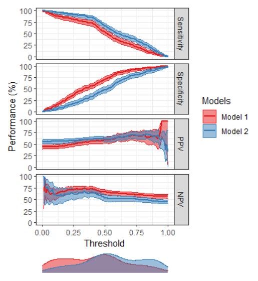
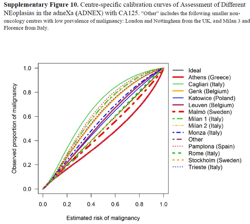
Large external validation

Van Calster et al. BMJ 2020;370:m2614. 58

Large external validation

• 4905 patients, 2012-2015, 17 centers

• First large study on the REAL population: any new patient with an
 ovarian tumor, whether operated or not (2489 were operated)

• If not operated, patients are followed conservatively. Then, outcome was
 based on clinical and ultrasound information.
 o Differential verification!

 o If insufficient or inconsistent FU information: missing data (MI)

 59

Large external validation: discrimination

• AUC
 o Analysis based on logit(AUC) and its SE (Snell 2019) – auRoc package
 o Random effects meta-analysis – metafor package, rma and predict functions
 o 95% prediction interval

• Calibration
 o One-stage calibration model for calibration intercept and slope
 o We used this model for calibration curves (i.e. no flexible calibration curves)
 o Overall curve: and set to 0
 o Center-specific curves: random terms used

 60

Large external validation: utility

• Decision: referral for specialized oncological care
• Reasonable range of risk thresholds: 5 to 50%

• Per threshold, Net Benefit per center was combined using Bayesian
 trivariate random effects meta-analysis
• Weak realistic priors
• WinBugs

 61

Large external validation: results

 62

Large external validation: results

 63

Large external validation: results

 64

Large external validation: results

 65

Large external validation: results

 66

Large external validation: results

 67

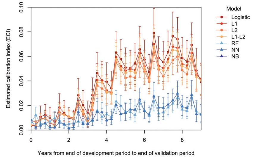
Large external validation: subgroups

 Operated (n=2489) At least 1 FU visit (n=1958)
 38% malignant 1% malignant

 68

Large external validation: subgroups

 Oncology centers (n=3094) Other centers (n=1811)
 26% malignant 10% malignant

 (Interestingly, LR2 (blue line) is the only model without type of center as a predictor)

 69

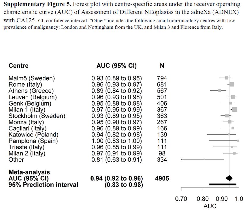
Large external validation: meta-regression
rma.uni(logit_auc, sei = se_logit_auc, mods = logit(EventRate), data = iota5cs, method = "REML", knha=TRUE)

 R2 42% R2 34%
 p 0.02 p 0.04

 R2 11% R2 16%
 p 0.24 p 0.09

 70

Large external validation: meta-regression
 rma.uni(lnOE, sei = se_lnOE, mods = logit(EventRate), data = iota5cs, method = "REML", knha=TRUE)

 R2 41% R2 0%
 p 0.29 p 0.50

 R2 0% R2 0%
 p 0.52 p 0.31

 71

Independent external validation studies
Study Location N ER AUC Calibration Utility Missing Reporting guideline
 (%) Data mentioned
Joyeux 2016 Dijon/Chalon (FR) 284 11 0.938 No No CCA None

Szubert 2016 Poznan (PL) 204 34 0.907 No No CCA None

 Pamplona (SP) 123 28 0.955 No No CCA None

Araujo 2017 Sao Paulo (BR) 131 52 0.925 No No CCA STARD

Meys 2017 Maastricht (NL) 326 35 0.930 No No MI STARD

Chen 2019 Shanghai (CN) 278 27 0.940 No No CCA None

Stukan 2019 Gdynia (PL) 100 52 0.972 No No CCA STARD, TRIPOD

Jeong 2020 Seoul (KR) 59 17 0.924 No No No info None

Viora 2020 Turin (IT) 577 25 0.911 No No CCA None

Nam 2021 Seoul (KR) 353 4 0.920 No No No info None

Poonyakanok 2021 Bangkok (TH) 357 17 0.975 No No CCA None

 72

Independent external validation studies
metagen(logitc, logitc_se, data = adnex, studlab = Publication, sm = "PLOGIT", backtransf = T,
 level = 0.95, level.comb = 0.95, comb.random = T, prediction = T, level.predict = 0.95,
 method.tau = "REML", hakn = TRUE)

 73

Heterogeneity?

 74

4. Machine learning

Regression vs Machine Learning

Breiman. Stat Sci 2001;16:199-231. 76

Regression vs Machine Learning

 ??

Shmueli. Keynote talk at 2019 ISBIS conference, Kuala Lumpur; taken from slideshare.net
Bzdok. Nature Methods 2018;15:233-4. 77

Reason for popularity

 “Typical machine learning algorithms are highly flexible

 So will uncover associations we could not find before

 Hence better predictions and management decisions”

 → One of the master keys, with guaranteed success!

 78

1. Study design trumps algorithm choice

 Do you have a clear research question?
 Do you have data that help you answer the question?
 What is the quality of the data?

 One simple example: EHR data were not collected for research purposes

Dilbert.com
Riley. Nature 2019;275:27-9. 79

Example

 Uses ANN, Random Forests, Naïve Bayes, and Logistic Regression.
 (Logistic regression performed best, AUC 0.92)

Hernandez-Suarez et al. JACC Cardiovasc Interv 2019;12:1328-38. 80

Example (contd)

 The model also uses postoperative information.
 David J Cohen, MD: “The model can’t be run properly until you know about both the presence and the absence of
 those complications, but you don’t know about the absence of a complication until the patient has left the hospital.”

https://www.tctmd.com/news/machine-learning-helps-predict-hospital-mortality-post-tavr-skepticism-abounds 81

Example 2

Winkler et al. JAMA Dermatol 2019; in press. 82

Example 3

Khazendar et al. Facts Views Vis ObGyn 2015;7:7-15. 83

2. Flexible algorithms are data hungry

http://www.portlandsports.com/hot-dog-eating-champ-kobayashi-hits-psu/ 84

Flexible algorithms are data hungry

Van der Ploeg et al. BMC Med Res Methodol 2014;14:137. 85

Flexible algorithms are data hungry

https://simplystatistics.org/2017/05/31/deeplearning-vs-leekasso/
Marcus. arXiv 2018; arXiv:1801.00631 86

3. Signal-to-noise ratio (SNR) is often low
 There is support that flexible algorithms work best with high SNR, not with low
 SNR.

 How can methods that look everywhere be better when you do not know
 where to look or what you look for?

Hand. Stat Sci 2006;21:1-14. 87

Algorithm flexibility and SNR

Ennis et al. Stat Med 1998;17:2501-8.
Goldstein et al. Stat Med 2017;36:2750-63.
Makridakis et al. PLoS One 2018;13:e0194889. 88

So I find this hard to believe

Rajkomar et al. NEJM 2019;380:1347-58. 89

What if you don’t know?

 If you have no knowledge on what variables could be good
 predictors (and what variables not), are you ready to make a
 good prediction model?

 I do not think that using flexible algorithms will bypass this.

 I like a clear distinction between
 - predictor finding studies
 - prediction modeling studies

 90

Machine learning: success guaranteed?
• Question 1: which algorithm works when?
 o Medical data: often limited signal:noise ratio
 o High-dimensional data vs CPM
 o Direct prediction from medical images using DL: different ballgame?

• Question 2: ML for low-dimensional CPMs?

 91

ML vs LR: systematic review

Christodoulou et al. J Clin Epidemiol 2019;110:12-22. 92

ML vs LR: systematic review

Christodoulou et al. J Clin Epidemiol 2019;110:12-22. 93

ML vs LR: systematic review

Christodoulou et al. J Clin Epidemiol 2019;110:12-22. 94

ML vs LR: systematic review

Christodoulou et al. J Clin Epidemiol 2019;110:12-22. 95

Poor modeling and unclear reporting

 What was done about missing data? 45% fully unclear, 100% poor or unclear

 How were continuous predictors modeled? 20% unclear, 25% categorized

 How were hyperparameters tuned? 66% unclear, 19% tuned with information

 How was performance validated? 68% unclear or biased approach

 Was calibration of risk estimates studied? 79% not at all, HL test common

 Prognosis: time horizon often ignored completely

Christodoulou et al. J Clin Epidemiol 2019;110:12-22. 96

ML vs LR: comparison of AUC

Christodoulou et al. J Clin Epidemiol 2019;110:12-22. 97

A few anecdotic observations

Christodoulou et al. J Clin Epidemiol 2019;110:12-22. 98

Conclusions

Validation is important, but there is no such thing as a validated model.

Expect and address heterogeneity in model development and validation.

Ideally, models should be locally and dynamically updated. Realistic?

Study methodology trumps algorithm choice.

Machine learning: no success guaranteed.

Reporting is key. TRIPOD extensions are underway (Cluster and AI).

 99

TG6 - Evaluating diagnostic tests and prediction models

Chairs: Ewout Steyerberg, Ben Van Calster

Members: Patrick Bossuyt, Tom Boyles (clinician), Gary Collins, Kathleen Kerr,
Petra Macaskill, David McLernon, Carl Moons, Maarten van Smeden, Andrew
Vickers, Laure Wynants

Papers:

- Van Calster et al. Calibration: the Achilles heel of predictive analytics. BMC Medicine 2019.

- Wynants et al. Three myths about risk thresholds for prediction models. BMC Medicine 2019.

- McLernon et al. Assessing the performance of prediction models for survival outcomes: guidance for
validation and updating with a new prognostic factor using a breast cancer case study. Near final!

- A few others in preparation.

 100