Classification of All-Rounders in the Game of ODI Cricket: Machine Learning Approach
←
→
Page content transcription
If your browser does not render page correctly, please read the page content below
Athens Journal of Sports - Volume 7, Issue 1, March 2020 – Pages 21-34

    Classification of All-Rounders in the Game of ODI
          Cricket: Machine Learning Approach
                            By Indika Wickramasinghe*
     Player classification in the game of cricket is very important, as it helps the
     coach and the captain of the team to identify each player’s role in the team and
     assign responsibilities accordingly. The objective of this study is to classify all-
     rounders into one of the four categories in one day international (ODI) Cricket
     format and to accurately predict new all-rounders’. This study was conducted
     using a collection of 177 players and ten player-related performance indicators.
     The prediction was conducted using three machine learning classifiers, namely
     Naive Bayes (NB), k-nearest neighbours (kNN), and Random Forest (RF).
     According to the experimental outcomes, RF indicates significantly better
     prediction accuracy of 99.4%, than its counter parts.

     Keywords: Team sport, machine learning, cricket, ODI, player classification

Introduction

     Cricket is considered as a bat and ball team game. The game has basically
three formats, namely, the test cricket, one-day-international cricket (ODI), and
T20. Test cricket, the longest format is regarded by experts of the game as the
ultimate test of playing skills. An ODI cricket game is played for 300 legal
deliveries (balls) per side, and the shortest format, T20 is played for 120 legal
deliveries (balls) per side. A typical cricket team comprises of 11 players and the
team batting first is identified by the outcome of tossing a coin. In the game of
cricket, there are three major disciplines: batting, bowling, and the fielding. When
selecting 11 players for a team, it is necessary to balancing the team by selecting
players to represent each of the above three departments.
     A player who excels in bowling the cricket ball is considered as a bowler,
while a player with higher potential of hitting the cricket ball is considered as a
batsman. An all-rounder is a regular performer with bat and the ball. According to
Bailey (1989), an all-rounder is a player who is able to grasp a position in his team
for either his batting or his bowling ability. Though fielding is an integral part in
the game, batting and bowling skills are given higher priorities than fielding. A
genuine all-rounder is a special all-rounder who is equally capable of batting and
bowling, most importantly this player can bat as a quality batsman and bowl as s
quality bowler. Majority of all-rounders in the game of cricket dominate either
batting or bowling skills, therefore they are named as batting all-rounders or as
bowling all-rounders.
     Identification of all-rounders is very vital for the success of a team. Classifying
an all-rounder as genuine, batting, or a bowling is even beneficial for cricket
selection panels, coaches, and players. A review at the literature provides evidences

*
 Assistant Professor, Department of Mathematics, Prairie View A&M University, USA.

https://doi.org/10.30958/ajspo.7-1-2                            doi=10.30958/ajspo.7-1-2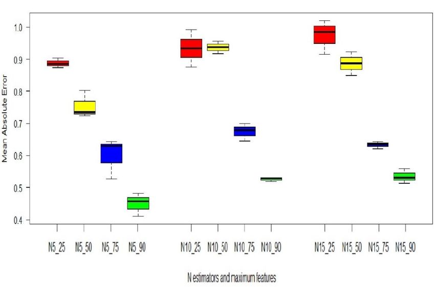
Vol. 7, No. 1     Wickramasinghe: Classification of All-Rounders in the Game of ODI…

of such studies. Using Indian Premier League (IPL) data, Saikia and Bhattacharjee
(2011) classified all-rounders into four groups, namely performer, batting all-
rounder, bowling all-rounder, and under-performer. According to their results, the
Naïve Bayes algorithm has given a classification accuracy of 66.7%. In an attempt
to rank all-rounders in test cricket, Tan and Ramachandran (2010) utilized both
batting and bowling statistics to devise a mathematical formula. In another study,
Stevenson and Brewer (2019) derived a Bayesian parametric model to predict how
international cricketers' abilities change between innings in a game. Furthermore,
Christie (2012) researched physical requirements of fast bowlers and stated the
necessity of physiological demands to evaluate bowlers’ performances. Saikia et
al. (2016) developed a performance measurement using a combination of batting
and bowling statistics to quantify all-rounder’s performance. Wickramasinghe (2014)
introduced an algorithm to predict batsman’s performance using a hierarchical
linear model. This multi-level model used player-level and team-level performance
indicators to predict the player’s performance.
     Selecting a team against a given opposition team is not an easy task, as
various aspects including the strengths and the weaknesses of both teams are
required to consider. Bandulasiri et al. (2016) identified a typical ODI game as a
mixture of batting, bowling, and decision-making. Presence of a quality all-
rounder in a team is an asset to a team, as it brings huge flexibility in the
composition of the team. A good all-rounder makes the captain’s job easy as the
player can play a dual role, whenever the captain requires (Van Staden 2008).
Though the impact of all-rounders towards the success of a team is enormous,
there are no underline criteria to identify them.
     The existence of prior research work in identifying all-rounders in the game
of cricket is handful. According to the knowledge of the author, there is no
existing study regarding classification of all-rounders in ODI format. Our
objective of this study is to device a method to categorize all-rounders in the ODI
format of cricket. We use several machine learning techniques to classify an all-
rounder as a genuine all-rounder, batting all-rounder, bowling all-rounder, and as
an average all-rounder.
     This study brings novelty for the cricket literature in many ways. According
to the author’s point of view, this is one of the first studies conducted to classify
all-rounders in ODI version of the game using machine learning techniques.
Furthermore, the selected player-related performance indicators and the used
machine learning techniques are unique for this study. Findings of this study can
benefit the entire cricket community and cricket industry as always prediction in
sports brings an economical value to the industry (Gakis et al. 2016).
     The rest of the manuscript is organized as follows. Next section will discuss
about the data selection procedure and descriptive statistics about the collected
data. In the methodology section, three machine learning techniques are discussed.
Then, in the following section findings of this study are illustrated. Finally, the
discussion and conclusion section will discuss further about the conducted study
and concludes the manuscript.

                                         22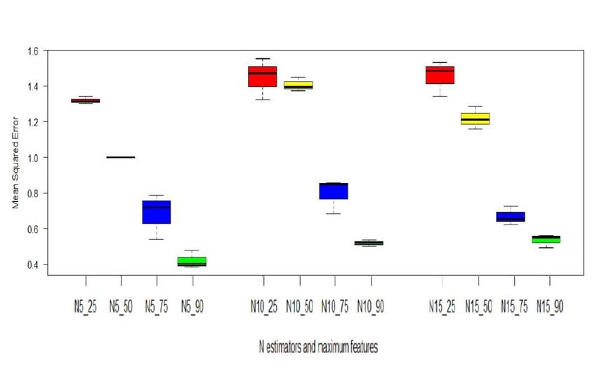
Athens Journal of Sports March 2020
Data Collection and Player - Selection Criteria
Data for this study was collected using a publically available website, under
the following criteria. Players, who have played more than 50 ODI games with an
aggregate score of over 500 runs, were selected. Furthermore, it was essential for
each player to have at least a half-century under their name, and collected more
than 25 ODI wickets. Under the above criteria, a total of 177 players were selected
and ten player related performance indicators (features) were recorded. Table 1
summarises these ten features and their descriptive statistics.
Table 1. Descriptive Statistics of Dataset
Variable Description Mean SD
Matches: The number of games each player has played 146.64 83.12
Number of accumulated runs a player has
Runs: 2,972.79 2,859.03
scored in his career
HS: Highest score a player has scored in his career 101.25 36.97
BatAv: Batting average of a player 26.04 9.12
Number of times a player has scored 100 runs
NumCen: 2.96 6.00
or more in a game
Number of accumulated wickets a player has
NumWkts: 115.79 86.05
taken in this career
BesstB: Best bowling figures as a bowler 4.51 0.98
BowAv: Bowling average of the bowler 35.04 6.64
Number of times a bowler has taken 5 or more
NFiveWkts: 0.99 1.58
wickets in a game
Number of catches a player has caught in his
NCatches: 47.32 30.83
career
Saikia and Bhattacharjee (2011) classified all-rounders based on median value
of both batting average and bowling averages. In this collected data, the
distributions of both batting and bowling follow Gaussian distributions. Therefore,
in this study we use the mean values of both batting and bowling averages to
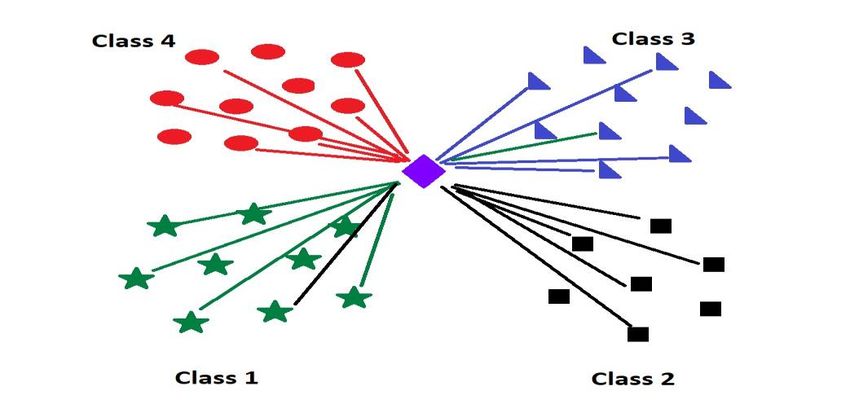
classify all-rounders according to the scheme summarised in Table 2. Figure 1
illustrates the joint distribution of batting and bowling averages, and the four
categories of players.
Based on the Table 2 and Figure 1, we classify each all-rounder into one of
the four categories: genuine all-rounder (G), batting all-rounder (B), bowling all-
rounder (Bw), and average all-rounder (A).
23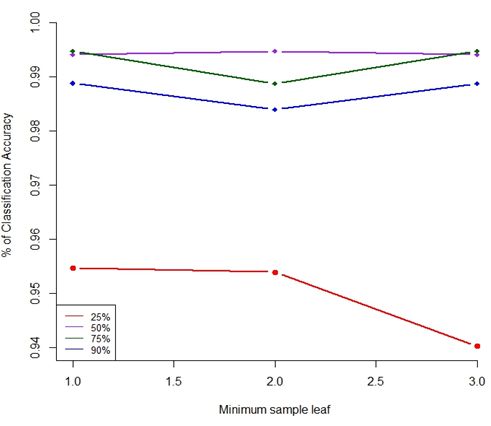
Vol. 7, No. 1 Wickramasinghe: Classification of All-Rounders in the Game of ODI…
Figure 1. Distribution of Batting Averages and Bowling Averages
Table 2. Classification Criteria of All-Rounders
Category of the all-rounder Criteria
(Type) Batting Average Bowling Average
Genuine (G) 26.04 35.04
Batting (B) 26.04 35.04
Bowling (Bw) 26.04 35.04
Average (A) 26.04 35.04
The class variable of the data set is named as Type, which represents each of the four classifications.
Methodology
In this study, we use three machine learning techniques, NB, kNN, and RF to
classify all-rounders into one of the four groups. Regression analysis is one of the
alternative conventional statistical procedures for an analysis like this. The number
of data appoints used in regression analysis is higher, proportional to the number
of involved features (Allision 1999, Bai and Pan 2009). Furthermore, some of the
machine learning algorithms such as NB is considered as a better performer with
smaller datasets (Hand 1992, Kuncheva 2006). Under the previously stated
constraints, we opt to use these three machine learning approaches to analyse these
data.
24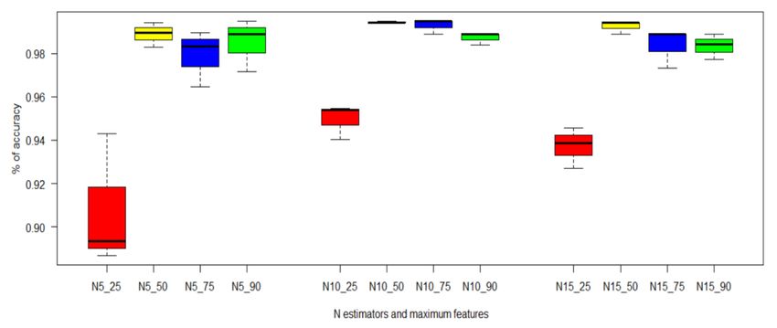
Athens Journal of Sports March 2020
Naïve Bayes (NB)
The NB classifier is considered as one of the simplest and accurate data
classifying algorithms. The base of this classifier is the well-known Bayes
theorem, used in probability theory. The simplicity, the accuracy, and the
robustness of NB have made NB a popular classifying technique with various
applications (Arar and Ayan 2017). As the literature indicates, NB is one of the top
performing classifiers used in data mining (Wu et al. 2008).
Let X x1 , x2 ,..., xn be a n-dimensional random vector (features) from domain
DX and Y ( y1 , y2 ,...., ym ) be a m-dimensional vector (classes) from domain DY .
In this study, n 10 is the number of factors and x1 , x2 ,..., x10 , the first column of the
Table 1. Similarly, here m 4 and Y ( y1, y2 , y3 , y4 ) ; y1 Genuine all rounder ,
y2 Batting all rounder , y3 Bowling all rounder, y4 Average all rounder .
Our aim is to estimate the value of Y by maximizing P Y y | X x . NB
assumes that features are independent of each other for a given class. Therefore,
P( X1 x1 , X 2 x2 ,..., X n xn | Y y)
P( X1 x1 | Y y).P( X 2 x2 | Y y)....P( X n xn | Y y)
i 1 P( X i xi | Y y )
n
.
P( X | y ) P( y )
According to the Bayes theorem, we have P y | X .
P( X )
Then we can write P y | X as follows.
P ( X x, Y y )
P y | X
P( X x)
P(Y y ) P ( X x | Y y )
P( X x)
P(Y y ) i 1 P ( X i xi | Y y )
n
n
i 1
P( X i xi )
P(Y y )
n
i 1
P ( X i xi | Y y )
Therefore, our aim is to find y, that maximize the above expression. In
another words, we need to find y, which is
arg max y P(Y y ) P(Y y ) i 1 P( X i xi | Y y )
n
25Vol. 7, No. 1 Wickramasinghe: Classification of All-Rounders in the Game of ODI…
k-Nearest Neighbour’s Algorithm (kNN)
The kNN can be considered as one of the simplest machine learning
classifiers, which is based on distance matric (Figure 2). Applications of kNN can
be found in text categorization (Elnahrawy 2002), ranking models (Xiubo et al.
2008), and object recognition (Bajramovic et al. 2006). If a novel data point is
given, kNN attempts to identify the correct category of the novel point, using the
characteristics of the neighbouring data points. The main trait of the data points is
going to be the distance from novel data point to each of the other data points.
When considering the distance metric, Euclidian is the most commonly used one
though other metrics such as Manhattan Distance, Mahalanobis Distance and
Chebychev Distances are also used in practice. Table 3 shows some other popular
distance matrices used in data classification.
Figure 2. kNN Classifier
Let {xi , yi }; i 1, 2,..., n be the training sample in which xi represents the
feature value and yi {c1 , c2 ,...., cM } represents the M categories (class value).
Furthermore, let X be a novel data point. The kNN algorithm can be summarised
as follows.
Calculating the distance from this novel point X to all other points in the
dataset.
Sort the distances from each point to the novel point and select the k
(usually an odd number to prevent tie situations) smallest distances, i.e.,
nearest k neighbours yi1 , yi 2 ,..., yik .
Then for each of the above k nearest neighbours, it records the
corresponding class (labels) c j ; j 1, 2,.., M and calculate the following
conditional probability.
26Athens Journal of Sports March 2020
P cx c j | X x
1 k
I c (x);
k i 1 i
1; x ci
where I ci ( x)
0; x ci
The class c j that has the highest probability is assigned to the novel data
point, as the category of the data point.
Table 3. Popular Distance Metrics
Name Distance Matric
x yi
n 2
Euclidean i 1 i
n
Manhattan i 1
| xi yi |
Chebyshev max | xi yi |
x yi
n p
Minkowski p
i 1 i
Random Forest (RF)
RF algorithm extends the idea of decision trees by aggregating higher number
of decision trees to reduce the variance of the novel decision tree (Couronné
2018). Each tree is built upon a collection of random variables (features) and a
collection of such random trees is called a Random Forest. Dues to the higher
classification accuracy, RF is considered as one of the most successful
classification algorithms in modern-times (Breiman 2001, Biau and Scornet 2016)
(Figure 3). Furthermore, the performance of this classification algorithm is
significant for unbalanced and missing data (Shah et al. 2014), compared to its
counterparts. RF has been studied by many researchers both in theoretically and
experimentally since its introduction in 2001 (Bernard et al. 2007, Breiman 2001,
Geurts 2006, Rodriguez 2006). Further studies have been conducted to improve
the classify-cation accuracy of RF by clever selection of the associated parameters
of RF (Bernard et al. 2007).
A handful of applications of machine learning algorithms in the context of
cricket can be seen in the literature. Using kNN and NB classifiers, Kumar and
Roy (2018) forecasted final score of an ODI score after the completion of the fifth
over of the game. NB and RF were two of the machine learning techniques Passi
and Pandey (2018) used in their study to predict the individual player’s
performance in the game of cricket. Using English T20 county cricket data from
2009 to 2014, Kampakis and Thomas (2015) developed a machine learning model
to predict the outcome of the T20 cricket game.
27Vol. 7, No. 1 Wickramasinghe: Classification of All-Rounders in the Game of ODI…
Figure 3. Random Forest Classifier
Dataset
subset subset subset
Tree Tree Tree
Findings
All the experimental outcomes were tested under the k-fold cross-validation,
which is used to generalize the findings of the study to any given independent
sample as discussed in the literature (Burman 1989, Kohavi 1995). We executed
all of the three machine learning classifiers with the collected data and according
to the experimental outcomes, NB classifier reached a maximum of 60.7%
prediction accuracy. Furthermore, the maximum prediction accuracy using Knn
was 55.08%. In order to see how the prediction accuracy changes with the
selection of distance matric with kNN algorithm, we measured the prediction of
accuracies with respect to the various distance matrices. Table 4 summarises the
percentage of prediction accuracy for each of the selected distance metric and the
value k used in kNN.
With RF, an initial accuracy rate of 93.34% was recorded, which is the
highest among the three classifiers we used. Further investigation was conducted
to optimize the prediction accuracy, by varying the associated parameters of RF.
28Athens Journal of Sports March 2020
Table 4. Distance Metric, K value, and Percentage of Prediction Accuracy
Distance Metric K Percentage of Accuracy
3 47.55%
Euclidian 5 49.36%
7 46.77%
3 49.81%
Manhattan 5 51.98%
7 54.83%
3 49.88%
Chebyshev 5 52.38%
7 55.08%
3 43.38%
Minkowski, p=3 5 50.99%
7 50.12%
Important Parameters used in RF
Among the various parameters used with RF, the following important
parameters were changed to see a better prediction rate.
n_estimators: This represents the number of trees in the RF.
max_features: This represents the maximum number of features when
the RF selects the split point.
min_samples_leaf: This represents how many minimum number of data
points in the end node.
Figure 4. Change of Prediction Accuracy with Different Parameters
Values of n_estimators, max_features, and min_samples_leaf were varied
from 5,10,15 , 0.25,0.50,0.75,0.90 , and {1, 2,3} . The obtained corresponding
values of the percentages of prediction accuracies are displayed by the Figure 4.
After searching for better parameterization, we investigated the associated
errors with the RF Regression model. Both Mean Absolute Error (MAE) and
Mean Squared Error (MSE) were recorded for the model with previously
identified parameters. Figures 6 and 7 display the variation of both MAE and MSE
29Vol. 7, No. 1 Wickramasinghe: Classification of All-Rounders in the Game of ODI…
for each values of parameters. As the experimental outcomes indicated, RF reached
a maximum prediction accuracy of 99.4% with the selection of n_estimators=10,
max_features=0.50, min_samples_leaf=2, and n_estimators=10, max_ features
=0.75, min_samples_leaf=1.
Figure 5. Prediction Accuracy, max_features and min_samples_leaf for n_
estimators=10
Figure 6. Parameters of Random Forest vs. Mean Absolute Error
30Athens Journal of Sports March 2020
Figure 7. Parameters of Random Forest vs. Mean Square Error
Discussion and Conclusion
In this manuscript, we discussed how to categorize all-rounders in the game of
ODI cricket. Using a collection of 177 players from all the ODI playing countries,
ten player-related predictors, together with three machine learning techniques, we
investigated how to categorize all-rounders into one of the four categories. In this
study, we utilized three machine learning techniques, namely Random Forest
(RF), k-nearest neighbours (kNN), and Naïve Bayes (NB) to predict the appropriate
category each of the all-rounder should belong.
After initial execution of the above three algorithms, the prediction accuracies
for kNN, NB, and RF were 50.08%, 59.00%, and 93.34% respectively. Further
improvement of the prediction accuracy was able to achieve with the proper
selection of the parameters. By changing the distance metric with kNN and the k
value, we were able to improve the prediction accuracy up to 55.08%. Similarly,
NB was improved up to 60.7%. According to Figures 4-7, it is clear that RF has
improved to the highest prediction accuracy of 99.4%, with the selection of
appropriate values for the parameters. This can be reached with two different
parameter settings. i.e., when n_estimators is 10, max_features is 0.50, min_
samples_leaf is 2, and n_estimators is 10, max_features is 0.75, min_samples_leaf
is 1. In addition to the prediction accuracy, an investigation was conducted to find
out the relative errors involved with these processes. According to the findings,
these errors became minimum when n_estimators is 10, max_features is 0.75 and
min_samples_leaf is 1 respectively and the values were 0.68 and 0.86 respectively.
In summary, our experimental results indicated that RF algorithm
outperformed both kNN and NB by huge margins. The findings of this study
benefit the officials of the game of cricket and the players in many ways. Player
selection committees, coaches of teams, and even the players can utilize these
outcomes to identify appropriate all-rounders. It would be important to include
31Vol. 7, No. 1 Wickramasinghe: Classification of All-Rounders in the Game of ODI…
additional performance indicators, including statistics about the opposition teams
that the players play against for future studies.
References
Allision PD (1999) Multiple regression: a primer. Thousand oaks. CA: Pine Forge Press.
Arar OF, Ayan K (2017) A feature dependent Naive Bayes approach and its application to
the software defectprediction problem. Applied Soft Computing 59(Oct): 197-209.
Bai H, Pan W (2009) An application of a new multivariate resampling method to multiple
regression. Multiple Linear Regression Viewpoints 35(1): 1-5.
Bailey T (1989) The greatest since my time. London: Hodder and Stoughton.
Bajramovic F, Mattern F, Butko N, Denzler J (2006) A comparison of nearest neighbor
search algorithms for generic object recognition. In J Blanc-Talon, W Philips, D
Popescu, P Scheunders (Eds.), Advanced Concepts for Intelligent Vision Systems.
ACIVS 2006. Lecture Notes in Computer Science, p. 4179. Berlin, Heidelberg: Springer.
Bandulasiri A, Brown T, Wickramasinghe T (2016) Characterization of the result of one
day format of cricket. Operation Research and Decisions 26(4): 21-32.
Bernard S, Heutte L, Adam S (2007) Using random forests for handwritten digit
recognition. 9th IAPR/IEEE International Conference on Document Analysis and
Recognition (ICDAR), Curitiba, Brazil. 1043-1047, ff10.1109/ICDAR.2007.437707
4ff.ffhal-00436372f.
Biau G, Scornet E (2016) A random forest guided tour. Test 25(2): 197-227. Doi:10.1007/
s11749-016-0481-7.
Breiman L (2001) Random forests. Machine Learning 45(1): 5-32.
Burman P (1989) A comparative study of ordinary cross-validation, v-fold cross-
validation and the repeated learning-testing methods. Biometrika 76(3): 503- 514.
Christie CJA (2012) The physical demands of batting and fast bowling in cricket. In KR
Zaslav (Ed.), An International Perspective on Topics in Sports Medicine and Sports
Injury: InTech, pp. 321-33.
Couronné R, Probst P, Boulesteix AL (2018) Random forest versus logistic regression: a
large-scale benchmark experiment. BMC Bioinformatics 19(1): 270. Doi:10.1186/s
12859-018-2264-5.
Elnahrawy E (2002) Log-based chat room monitoring using text categorization: a
comparative study. In St Thomas (Ed.), Proceedings of the IASTED International
Conference on Information and Knowledge Sharing (IKS 2002). US Virgin Islands,
USA.
Gakis K, Parsalos P, Park J (2016) A probabilistic model for multi-contestant races.
Athens Journal of Sports 3(2): 111-118.
Geurts G, Ernst D, Wehenkel L (2006) Extremely randomized trees. Machine Learning
36(1): 3-42.
Hand DJ (1992) Statistical methods in diagnosis. Statistical Methods in Medical Research
1(1): 49-67.
Kampakis S, Thomas B (2015) Using machine learning to predict the outcome of English
county twenty over cricket matches. Arxiv: Machine Learning, 1-17.
Kohavi R (1995) A study of cross-validation and bootstrap for accuracy estimation and
model selection. Proceedings of the 14th Joint Conference on Artificial Intelligence
(IJCAI), vol. 2, 1137-1143.
32Athens Journal of Sports March 2020
Kumar S, Roy S (2018) Score prediction and player classification model in the game of
cricket using machine learning. International Journal of Scientific & Engineering
Research 9(8): 237-242.
Kuncheva LI (2006). On the optimality of Naıve Bayes with dependent binary features.
Pattern Recognition Letters 27(7): 830-837.
Passi K, Pandey N (2018) Increased prediction accuracy in the game of cricket using
machine learning. International Journal of Data Mining & Knowledge Management
Process 8(2): 19-36.
Rodriguez J, Kuncheva L, Alonso C (2006) Rotation forest: A new classifier ensemble
method. IEEE Transactions on Pattern Analysis and Machine Intelligence 28(10):
1619-1630.
Saikia H, Bhattacharjee D (2011) On classification of all-rounders of the Indian premier
league (IPL): a Bayesian approach. Vikalpa 36(4): 51-66. 10.1177/02560909201104
04.
Saikia H, Bhattacharjee D, Radhakrishnan UK (2016) A new model for player selection in
cricket. International Journal of Performance Analysis in Sport 16(Apr): 373-388.
Shah AD, Bartlett JW, Carpenter J, Nicholas O, Hemingway H (2014) Comparison of
random forest and parametric imputation models for imputing missing data using
mice: a caliber study. American Journal of Epidemiology 179(6): 764-774. https://
doi.org/10.1093/aje/kwt312.
Stevenson OG, Brewer BJ (2019) Modelling career trajectories of cricket players using
Gaussian processes. In R Argiento, D Durante, S Wade (Eds.), Bayesian Statistics
and New Generations. BAYSM 2018. Springer Proceedings in Mathematics &
Statistics, vol. 296. Springer, Cham.
Tan A, Ramachandran R (2010) Ranking the greatest all-rounders in test cricket. Available
at: www.cricketsociety.com/ranking_the_greatest_all-ro.pdf.
Van Staden PJ (2008) Comparison of bowlers, batsmen and all-rounders in cricket using
graphical display. Technical Report 08/01. Department of Statistics, University of Pretoria,
South Africa.
Wickramasinghe IP (2014) Predicting the performance of batsmen in test cricket. Journal
of Human Sport & Exercise 9(4): 744-751.
Wu X, Kumar V, Quinlan R, Ghosh J, Yang Q, Motoda H, McLachlan J, Ng A, Liu B,
Yu PS, Zhou Z, Steinbach M, Hand DJ, Steinberg D (2008) Top 10 algorithms in
data mining. Knowledge and Information Systems 14(1): 1-37.
Xiubo G, Liu T, Qin T, Arnold A, Li H, Shum H (2008) Query dependent ranking using
K-nearest neighbor, Proceedings of the 31st Annual International ACM SIGIR
Conference on Research and Development in Information Retrieval. Singapore.
Doi:10.1145/1390334.1390356.
33Vol. 7, No. 1 Wickramasinghe: Classification of All-Rounders in the Game of ODI…
34You can also read