Space evaluation in football games via field weighting based on tracking data - Nature
←
→
Page content transcription
If your browser does not render page correctly, please read the page content below
www.nature.com/scientificreports
OPEN Space evaluation in football
games via field weighting based
on tracking data
Takuma Narizuka1*, Yoshihiro Yamazaki2 & Kenta Takizawa1
In football game analysis, space evaluation is an important issue because it is directly related to the
quality of ball passing or player formations. Previous studies have primarily focused on a field division
approach wherein a field is divided into dominant regions in which a certain player can arrive prior to
any other players. However, the field division approach is oversimplified because all locations within a
region are regarded as uniform herein. The objective of the current study is to propose a fundamental
framework for space evaluation based on field weighting. In particular, we employed the motion
model and calculated a minimum arrival time τ for each player to all locations on the football field.
Our main contribution is that two variables τof and τdf corresponding to the minimum arrival time
for offense and defense teams are considered; using τof and τdf , new orthogonal variables z1 and z2
are defined. In particular, based on real datasets comprising of data from 45 football games of the J1
League in 2018, we provide a detailed characterization of z1 and z2 in terms of ball passing. By using
our method, we found that z1 ( x , t) and z2 (
x , t) represent the degree of safety for a pass made to x at
t and degree of sparsity of x at t, respectively; the success probability of passes could be well-fitted
using a sigmoid function. Moreover, a new type of field division approach and evaluation of ball
passing just before shots using real game data are discussed.
The game of football, which is also commonly referred to as soccer, is a complex system wherein 22 players in
two different teams interact with each other in order for their team to win. In the process of carrying a ball to
their respective goal, a vast number of movement options are available to players, leading to the emergence of
various behaviors from individual to team levels, such as ball passing, dribbling, marking an opponent player,
and organizing into formations. The emergence of such behaviors in football, and recent developments in data
acquisition methodologies and tools1 have promoted a wide range of analyses for football games from the per-
spective of statistics as well as physics2,3. Examples of such analyses include the universality of goal distribution4,
complex network analysis for ball passing5,6, dynamics-based analysis of ball m otion7,8, and characterization of
formations9,10 . (We refer to a term, “formation”, as the relative positioning of players expressed in a form such
as 4–4–3).
In football games, the difficulty of receiving a pass or making a shot depends on the players’ formations or
the position of the ball. It is natural to assume that each location on the field has some value related to the game
condition. Thus characterization of space on the field by such a value is a key issue in football game analysis.
However, the definition of space in the context of football is not well-defined and neither are approaches for its
evaluation. In general, there are two approaches for space evaluation, namely field division and field weighting.
A well-known approach for field division is determining a “dominant region”—as introduced by Taki et al.11,12—
wherein a certain player can arrive in a region prior to any other players. A typical example of field division
is defining a Voronoi region for each player, which corresponds to their dominant region as defined by the
Euclidean distance between their position and each location in the field13. The Voronoi region provides a first
approximation of the territory of any player on the field. Previous studies have investigated its basic properties
in football games; for example, Kim have characterized the area and number of vertices of Voronoi regions14 and
Fonseca et al. have performed a time series analysis for Voronoi r egions15.
However, because these Voronoi regions lack information about the velocity and acceleration of players,
Fujimura and Sugihara proposed a more realistic definition of the dominant region based on a “motion model”16.
In the motion model, each player is assumed to move according to an equation of motion with acceleration and
resistance terms. Thus, given the initial position and velocity of a player, their arrival times at any location on
1
Department of Physics, Faculty of Science and Engineering, Chuo University, Bunkyo, Tokyo 112‑8551,
Japan. 2Department of Physics, School of Advanced Science and Engineering, Waseda University, Shinjuku,
Tokyo 169‑8555, Japan. *email: pararel@gmail.com
Scientific Reports | (2021) 11:5509 | https://doi.org/10.1038/s41598-021-84939-7 1
Vol.:(0123456789)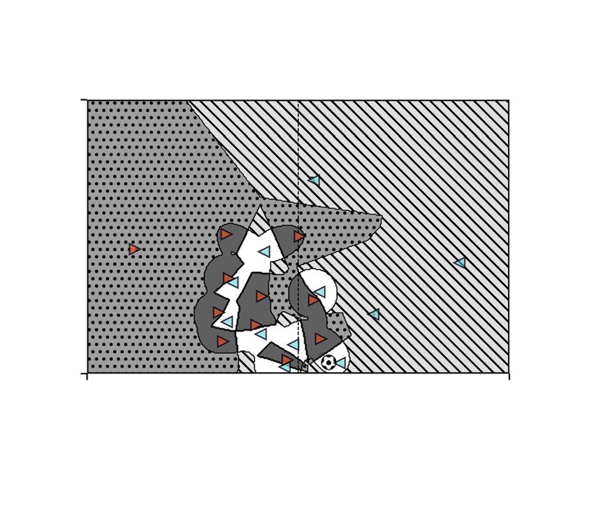
www.nature.com/scientificreports/
the field can be calculated based on the equation of motion. Accordingly, using the equations of motion, the
Voronoi regions of players can be suitably modified as per their velocity and acceleration. Using the motion
model, Fujimura and Sugihara have investigated the receivable pass variation which quantifies the number of
passes a player can r eceive16 and Ueda et al. have examined the relationship between the dominant region and
offensive performance of a t eam17. Another approach for extension of the definition of a dominant region is a
data-driven one wherein individual dominant regions on the field could be estimated using machine learning18,19.
Though field division based on dominant regions is one approach for space evaluation when positions and
motions of players are known, it is an oversimplified approach, because all locations within a dominant region
yield the same space evaluation in that only one specific player can reach a location first. For further detailed
characterization of space, the field division approach could be replaced by a field weighting approach using
appropriate variables. Several recent studies have addressed the problem of field weighting based on variables
such as pass p robability20, scoring opportunity21, and space occupation and generation g ain22. However, a field
weighting using arrival times of players could extend the field division approach in a more straightforward way.
In this study, we proposed a framework for space evaluation based on field weighting, which provides a defi-
nition of space from a new perspective. In particular, our space evaluation approach is based on a “minimum
arrival time” τ to all locations in the field, which can be calculated based on the physics-based motion model.
Herein, we considered two variables τof and τdf corresponding to the minimum arrival time for offense and
defense teams, respectively. Using τof and τdf , we introduced new orthogonal variables z1 and z2 that represent
degrees of safety and sparsity of each location, respectively. To elucidate the quantitative meaning of z1 and z2,
we carried out ball-passing analyses based on real datasets. As applications of our proposed space evaluation
method, a new field division approach is discussed and an evaluation of ball passing just before shots for a dataset
of football games is presented.
Methods
Dataset and system. The following characterization and demonstration of our space evaluation frame-
work was based on datasets comprising data from 45 football games of the top division of the J League in 2018;
these datasets were provided by DataStadium Inc., Japan23. This top division consists of 18 teams, then 9 games
are performed in one section. We had the dataset of five sections, therefore 45 games, which were held between
Aug. 10, 2018 and Sept. 2, 2018. We note that J League stands for the Japan Professional Football League, and
it has now matured enough to attract top players from all over the world. Each dataset contains information
about the absolute positional coordinates (x, y) of all players every 0.04 s as well as play-by-play data; the spatial
resolution of the data is on the centimeter scale. DataStadium Inc. was authorized to collect and sell this data
under a contract with the J League. This contract also ensures that the use of relevant datasets does not infringe
on any rights of the players and clubs belonging to the J League. Though the datasets are proprietary, we received
explicit permission from DataStadium Inc. for their use in this research. The data analyses and visualizations in
this study were performed using Python packages on a MacBook Pro system with a 2-GHz Intel Core i5 proces-
sor and 16 GB of memory.
Motion model. Here, we summarize the motion model proposed by Fujimura and Sugihara, which is also
used in this s tudy16. In this motion model, each player is assumed to move according to the following equation
of motion:
d 2 x� (t) d�x (t)
m = F n� − k (1)
dt 2 dt
where m is the mass of the player and x (t) is the position of the player at time t; F and n are the magnitude and
direction of the attractive force, respectively; and k is the coefficient for viscous resistance. Namely, we assume
that the player accelerates in the direction of n with magnitude F and becomes harder to accelerate in propor-
tion to its velocity d x (t)/dt . The solution for Eq. (1) for an initial position x 0 and initial velocity v 0 is expressed
as follows:
1 − exp(−αt) 1 − exp(−αt)
x� (t) = x�0 + v�0 + Vmax t − n� , (2)
α α
where Vmax = F/m and α = k/m are arbitrary constants that correspond to the player’s terminal velocity and
the inverse of the relaxation time to Vmax , respectively. Thus, given Vmax and α, we can obtain arrival times of
each player to all locations using Eq. (2). In the study by Fujimura and Sugihara, they set Vmax = 7.8 [m/s] and
α = 1.3 [1/s]; these values have been used for typical values during sprinting by the players and do not vary
significantly among p layers16.
Results
Definition of variables. Let τa ( x , t) be the minimum arrival time for a player a to a location x at time t.
Accordingly, τa ( x , t) is defined as the minimum time required for the player a to move from their position at t
to x . In order to calculate τa ( x , t), we employed the solution of the aforementioned motion model (i.e., Eq. 2).
For simplicity, we set Vmax = 7.8 [m/s] and α = 1.3 [1/s] for all players by assuming that they move to all loca-
tions by sprinting. This simplification is considered appropriate for grasping the essential features of our space
evaluation framework (i.e., the characterization of the meanings of z1 and z2) because Vmax and α do not vary
significantly among players. However, for a more practical application of our framework such as assessing the
Scientific Reports | (2021) 11:5509 | https://doi.org/10.1038/s41598-021-84939-7 2
Vol:.(1234567890)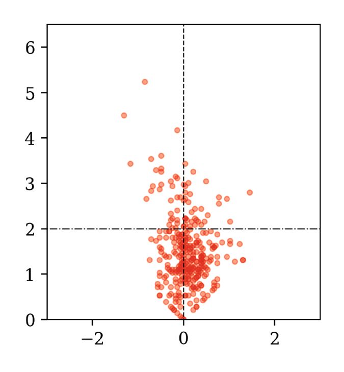
www.nature.com/scientificreports/
Figure 1. Visualization of τdf at a certain time as a contour plot over a range of 2 s. Players in offense (i.e., ball
possession team) and defense teams are depicted using blue leftward and red rightward triangles, respectively.
In this situation, the player on the right side near the halfway line has the ball and is trying to pass it to the other
side.
Figure 2. Relationship between the axes of τof and τdf and those of z1 and z2. The safe space (z1 > 0) and the
risky space ( z1 < 0) for the offense team are shown by shading.
playing ability of players, the use of more realistic values for Vmax and α based on the play in different games is
recommended.
Furthermore, we also define the minimum arrival time for a team A to x at time t as τA (�x , t) ≡ mina∈A τa (�x , t).
In particular, we denote the minimum arrival time for the defense and offense teams as τdf ( x , t) and τof ( x , t),
respectively; here, the offense team is defined as the team that has possession of the ball. Figure 1 depicts a visu-
alization for τdf at a certain time as a contour plot over a range of 2 s.
Now, we evaluate the location x at time t using the two variables τdf ( x , t) and τof ( x , t). In Fig. 2, the domain
τof ( x , t) < τdf ( x , t) corresponds to the “safe space” for the offense team in that an offense player can arrive in this
domain prior to any defense player. Thus, the degree of safety of x at t for the offense team can be quantified via
a signed distance z1 ( x , t) from the axis τof (�x , t) = τdf (�x , t) as follows:
τdf (�x , t) − τof (�x , t)
z1 (�x , t) = √ . (3)
2
When z1 > 0, τof < τdf . Therefore, an offense player can reach faster than a defense player at the space satisfying
z1 > 0. That is, the space for z1 > 0 is safe for the offense player. In Fig. 2, the safe space ( z1 > 0) and the risky
space ( z1 < 0) for the offense team are shown by shading. Similarly, another variable z2 ( x , t), which is orthogonal
to z1 ( x , t), can be defined as follows:
τdf (�x , t) + τof (�x , t)
z2 (�x , t) = √ . (4)
2
Scientific Reports | (2021) 11:5509 | https://doi.org/10.1038/s41598-021-84939-7 3
Vol.:(0123456789)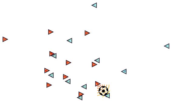
www.nature.com/scientificreports/
Figure 3. (a) Scatter plot of z1 ( xe , to ) and z2 ( xe , to ) for 34,189 passes obtained from 45 football games. Plots
for failed and successful passes almost distribute in z1 < 0 and z1 > 0 domains, respectively. (b) Probability
distributions of z1 ( xe , to ) for successful and failed passes. The dotted curves are the fitted normal distribution
curves. (c) Success probability of passes as a function of z1 ( xe , to ). The success probabilities are calculated by
averaging the value of q over each z1. The dotted curve is the fitted sigmoid function given by Eq. (5), indicating
that z1 ( x , t) signifies the degree of safety for a pass made to x at time t.
Because z2 ( x , t) is proportional to τdf + τof , the larger z2 ( x , t) is, the more time it takes for the players to reach
x . Therefore, z2 ( x , t) roughly quantifies the degree of sparsity of the location x at t. The relationship between the
axes of τof and τdf and those of z1 and z2 is depicted in Fig. 2. It is noteworthy that the definitions of z1 and z2
are independent of the definition of the motion model even though we employ the motion model proposed by
Fujimura and Sugihara for one specific case in this study.
Calculation of z1 and z2 using ball‑passing data. For further characterization of z1 and z2 using real-
world ball-passing data, we created time-series data using 34,189 ball passes made in 45 football games that form
part of the datasets used in our study. A row in the datasets corresponding to a pass is expressed as [to , x�o , te , x�e , q].
Here, to and x o represent the time and positional coordinates for the origin of the pass, while te and x e represent
those for the end of the pass, respectively. The variable q ∈ {1, 0} indicates the success (1) or failure (0) of a pass.
For each pass, we describe the state of the end of the pass ( x e) at the moment the pass is made (to) using z1 ( xe , to )
and z2 ( xe , to ). In order to investigate the relationship between the state of the end position and outcome of the
pass (success or failure), we calculated z1 ( xe , to ) and z2 ( xe , to ) for all successful and failed passes using Eqs. (3)
and (4), respectively; Fig. 3a shows the results of these calculations as a scatter plot.
Meaning of z1 (
xe , to ). Figure 3b presents the probability distributions of z1 ( xe , to ) for successful and
failed passes, which are denoted by P(z1 |q = 1) and P(z1 |q = 0), respectively. From the figure, we can observe
that both distributions can be fitted well using normal distribution functions. From the corresponding normal
curves, the mean and standard deviation for successful passes are obtained as µ1 = 0.69 and σ1 = 0.54, while
those for failed passes are µ0 = −0.25 and σ0 = 0.38. It is noteworthy that the peak values of these normal
curves—which correspond to the mean values—are located at z1 > 0 and z1 < 0 for successful and failed passes,
respectively. The sign of z1 ( xe , to ) depends on whether a player of the offense or defense teams reaches the ball
sooner. Thus, it is reasonable that the sign of µ is strongly correlated with the outcome of the pass. Furthermore,
we estimated the success probability P(q = 1|z1 ) of passes as a function of z1 ( xe , to ) by averaging the value of q
over each z1. Figure 3c shows our estimation results for the success probability of passes; from these results, it was
observed that these success probability values could be fitted well using a sigmoid function, which is given by:
1
P(q = 1|z1 ) = (5)
1 + exp[−(az1 + b)]
where a = 4.68 and b = 0.48. Thus, with respect to ball passing, z1 ( x , t) signifies the degree of safety for a pass
made to x at time t. In addition, this result suggests that the outcome of a particular pass can be estimated via
logistic regression using z1.
Meaning of z2 ( xe , to ). As mentioned earlier, z2 ( xe , to ) indicates the degree of sparsity of x e at to. To eluci-
date the meaning of sparsity, we calculate the following quantity for each pass:
||�xe − x�c (to )||
R̃ = . (6)
σ (to )
Here, x c is the centroid position for all 20 field players excluding the goal keepers; σ is the standard deviation
from x c , which corresponds to the size of the formation; these variables are defined as follows:
Scientific Reports | (2021) 11:5509 | https://doi.org/10.1038/s41598-021-84939-7 4
Vol:.(1234567890)www.nature.com/scientificreports/
Figure 4. (a) Schematic representation of the definition of R̃ (Eq. 6). Players in two teams are represented by
red rightward and blue leftward triangles. The cross and star markers represent the end points of x c (to ) and x e,
respectively. The dotted line indicates the circle with radius σ (to ). This case corresponds to R̃ > 1, meaning that
the end point of the pass is located outside the formation. (b) Relationship between R̃ and z2 ( xe , to ). z2 (�x , t) ≃ 2
is the threshold that determines whether the location x at t is inside or outside the formation. We roughly regard
the spaces with z2 2 and z2 2 as sparse and dense, respectively.
20
1
x�c (t) = x�j (t), (7)
N
j=1
20
1
σ (t) =
|�xc (t) − x�j (t)|2 . (8)
20
j=1
Figure 4a shows the schematic representation of the definition of R̃ . When R̃ is less (more) than unity, the end
point x e of the pass is roughly located inside (outside) the formation.
The relationship between R̃ and z2 obtained based √ on our data is shown in Fig. 4b. It was observed that the
value of z2 at which R̃ ≃ 1 is ≃ 2, i.e., τdf + τof ≃ 2 2 ; thus, z2 (�x , t) ≃ 2 is the threshold that determines whether
the location x at t is inside or outside the formation. Based on this result, we roughly regard the spaces with
z2 2 and z2 2 as sparse and dense spaces, respectively.
Discussion
The objective of the current study was to propose a fundamental framework for space evaluation based on
field weighting. The properties and significance of our proposed framework for space evaluation are described
below. First, instead of a field division approach, our framework is based on a field weighting approach derived
from a previous motion model. Second, the variables for field weighting have an explicit physical meaning, i.e.,
minimal arrival times of players when they move to all locations by sprinting. Third, each location is evaluated
using two variables; τdf and τof , and the influence of both the defense and offense teams at each location can be
simultaneously evaluated using our approach. Fourth, most importantly, two orthogonal variables z1 and z2 ,
which correspond to the degrees of safety and sparsity of a location, were introduced. It is important to note that
our framework does not depend on the definition of a motion model; in addition, z1 and z2 provide a quantitative
definition of space on the football field. Therefore, our framework essentially yields a starting point to answer
the question, “what is space in football games?”
Based on the ball-passing analysis discussed above, our framework also provides a new approach for field
division based on the degrees of safety and sparsity. In particular, using the two axes, z1 = 0 and z2 = 2, the
football field can be divided into the following four spaces: (A) safe dense space ( z1 > 0 and z2 < 2), (B) safe
sparse space ( z1 > 0 and z2 > 2), (C) risky sparse space ( z1 < 0 and z2 > 2), and (D) risky dense space ( z1 < 0
and z2 < 2). We show a typical example of field division using our approach into spaces (A)–(D) in Fig. 5. From
the figure, it can be confirmed that the dense spaces (A) and (D) defined as z2 < 2 are almost located within the
formation, i.e., R̃ < 1.
For example, in the case shown in Fig. 5, the player on the right side near the halfway line has the ball. In
order for this player to execute a shot from this location, the ball has to be sent to a space in front of the oppo-
nent’s goal; however, this space is risky because it corresponds to (C) or (D). We show that passes just before
shots have a tendency to become risky generally based on our framework. For passes just before shots, Fig. 6a,b
present the scatter plots for z1 ( xe , to ) and z2 ( xe , to ), and the probability distribution of z1 for successful passes,
respectively. From Fig. 6b, we can observe that the peak value z1 ≃ 0 is smaller than that for the case of all passes
( z1 = 0.69 in Fig. 3b). This observation indicates that passes just before a shot tend to become risky because
the success probability of a pass is a monotonically increasing function of z1, as shown in Fig. 3c. Here, Fig. 6
Scientific Reports | (2021) 11:5509 | https://doi.org/10.1038/s41598-021-84939-7 5
Vol.:(0123456789)www.nature.com/scientificreports/
Figure 5. Typical example of field division into the following four spaces: (A) safe dense space (z1 > 0 and
z2 < 2), (B) safe sparse space (z1 > 0 and z2 > 2), (C) risky sparse space (z1 < 0 and z2 > 2), and (D) risky
dense space (z1 < 0 and z2 < 2). The players in the offense (i.e., ball-possession team) and defense teams are
shown via blue leftward and red rightward triangles, respectively. The player on the right side near the halfway
line has the ball. In order for this player to execute a shot from this location, the ball has to be sent to a space in
front of the opponent’s goal; however, this space is risky because it corresponds to (C) or (D).
Figure 6. (a) Scatter plot of z1 ( xe , to ) and z2 ( xe , to ), and (b) probability distribution of z1 ( xe , to ), for successful
passes just before the shots.
shows an average feature for various teams. Examining the same figure for an individual team will lead to team
assessment in terms of the shot situation. For example, from the peak position in Fig. 6b for each team, we can
evaluate how risky they are in shot situations.
As shown in Fig. 3c, the success probability P(q = 1|z1 ) of passes being well-fitted by the sigmoid function (5)
could be a consequence of the normal distributions for P(z1 |q = 1) and P(z1 |q = 0) (see Fig. 3b). In particular,
it is known that P(q = 1|z1 ) can be expressed as follows:
1
P(q = 1|z1 ) =
,
P(z |q=1)P(q=1)
1 + exp − log P(z11 |q=0)P(q=0)
which transforms to Eq. (5) when P(z1 |q = 1) and P(z1 |q = 0) follow a normal distribution with the same stand-
ard deviation24. In our case, the standard deviations obtained from fitting our data are σ1 = 0.54 and σ0 = 0.38,
and σ1 = σ0. The deviation of the success probability curve shown in Fig. 3c from the sigmoid function curve
where z1 < 0 can be attributed to this difference in standard deviation values. The sigmoid curve for z1 can be
applied to the player assessment in terms of difficulty of ball passings. For example, a player who completed
many passes with z1 < 0 can be evaluated as a good passer because such passes are difficult to complete by the
sigmoid curve. In particular, σ1 and σ2 may be related to the passing abilities of players. Thus, new criteria for
pass evaluation can be a typical practical application of our framework.
Finally, here, we present directions for future research related to the present study by comparing our frame-
work with other relevant studies. First, Fernández and Bornn proposed a field weighting approach for space
evaluation in football games22. In their method, a player’s influence on each location is defined by a multivariate
normal distribution and is transformed into a single value to evaluate which team is dominant at a location. In
contrast, our method evaluates a location in the field based on two variables, z1 and z2, which are defined based
on the motion model. It is noteworthy that each of z1 ( x , t) and z2 ( x , t) has an explicit physical meaning, i.e., the
degree of safety for a pass made to x at t and degree of sparsity of x at t, respectively. Several extensions to our
Scientific Reports | (2021) 11:5509 | https://doi.org/10.1038/s41598-021-84939-7 6
Vol:.(1234567890)www.nature.com/scientificreports/
proposed framework are required before it can be applied to real game analyses. For example, the information
of the distances from the locations of the ball and goal should be incorporated into variables for field weighting
as in the case of Fernández and Bornn’s approach, because the outcome of passes or shots typically depends on
these distances. In regard to the motion of the ball, Spearman et al. proposed a model based on the equation
of motion for the b all20,21. Our proposed framework could also be similarly extended to the ball, which would
enable us to evaluate the accuracy of passes. Because our framework is independent of the definition of the
motion model, we could employ any extended motion model based on the equations of motion or machine
learning technique18,19 for calculating z1 and z2. A player-specific motion model might also allow us to assess
the playing ability of players.
Data availability
The dataset (Player Tracking Data in J-League Matches) was obtained from DataStadium Inc., Japan; it is not
publicly available, but it was provided to us based on an agreement with the company.
Received: 4 June 2020; Accepted: 23 February 2021
References
1. Pappalardo, L. et al. A public data set of spatio-temporal match events in soccer competitions. Sci. Data 6, 236 (2019).
2. Sumpter, D. Soccermatics: Mathematical Adventures in the Beautiful Game (Bloomsbury Sigma, 2016).
3. Gudmundsson, J. & Horton, M. Spatio-temporal analysis of team sports. ACM Comput. Surv. 50, 1–34 (2017).
4. Malacarne, L. & Mendes, R. Regularities in football goal distributions. Phys. A Stat. Mech. Appl. 286, 391–395 (2000).
5. Duch, J., Waitzman, J. S. & Amaral, L. A. N. Quantifying the performance of individual players in a team activity. PLoS ONE 5,
e10937 (2010).
6. Buldú, J. M., Busquets, J., Echegoyen, I. & Seirul-lo, F. Defining a historic football team: Using Network Science to analyze Guar-
diola’s F.C. Barcelona. Sci. Rep. 9, 1–14 (2019).
7. Mendes, R. S., Malacarne, L. C. & Anteneodo, C. Statistics of football dynamics. Eur. Phys. J. B 57, 357–363 (2007).
8. Kijima, A., Yokoyama, K., Shima, H. & Yamamoto, Y. Emergence of self-similarity in football dynamics. Eur. Phys. J. B 87, 41
(2014).
9. Bialkowski, A. et al. Large-scale analysis of soccer matches using spatiotemporal tracking data. in 2014 IEEE International Confer-
ence on Data Mining, 725–730 (2014).
10. Narizuka, T. & Yamazaki, Y. Clustering algorithm for formations in football games. Sci. Rep. 9, 1–8 (2019).
11. Taki, T., Hasegawa, J.-I. & Fukumura, T. Development of motion analysis system for quantitative evaluation of teamwork in soccer
games. Proc. 3rd IEEE Int. Conf. Image Process. 3, 815–818 (1996).
12. Taki, T. & Hasegawa, J.-I. Visualization of dominant region in team games and its application to teamwork analysis. Proc. Comput
Graph. Int. 2000, 227–235 (2000).
13. Okabe, A., Boots, B., Sugihara, K. & Nok-Chiu, S. Spatial Tessellations: Concepts and Applications of Voronoi Diagrams (Wiley,
2000).
14. Kim, S. Voronoi analysis of a soccer game. Nonlinear Anal. Model. Control. 9, 233–240 (2004).
15. Fonseca, S., Milho, J., Travassos, B. & Araújo, D. Spatial dynamics of team sports exposed by Voronoi diagrams. Hum. Mov. Sci.
31, 1652–1659 (2012).
16. Fujimura, A. & Sugihara, K. Geometric analysis and quantitative evaluation of sport teamwork. Syst. Comput. Jpn. 36, 49–58 (2005).
17. Ueda, F., Masaaki, H. & Hiroyuki, H. The causal relationship between dominant region and offense–defense performance—Focus-
ing on the time of ball acquisition. Footb. Sci. 11, 1–17 (2014).
18. Gudmundsson, J. & Wolle, T. Football analysis using spatio-temporal tools. Comput. Environ. Urban Syst. 47, 16–27 (2014).
19. Brefeld, U., Lasek, J. & Mair, S. Probabilistic movement models and zones of control. Mach. Learn. 108, 127–147 (2019).
20. Spearman, W., Basye, A., Dick, G., Hotovy, R. & Pop, P. Physics-based modeling of pass probabilities in soccer. in MIT Sloan Sports
Analytics Conference, 1–14 (2017).
21. Spearman, W. Beyond expected goals. in MIT Sloan Sports Analytics Conference, 1–17 (2018).
22. Fernández, J. & Bornn, L. Wide open spaces: A statistical technique for measuring space creation in professional soccer. in MIT
Sloan Sports Analytics Conference, 1–19 (2018).
23. DataStadium Inc. https://www.datastadium.co.jp/en/index.
24. Bishop, C. M. Pattern Recognition and Machine Learning (Springer, 2006).
Acknowledgements
The authors are grateful to DataStadium Inc., Japan, for providing the player tracking data for this study. This
work was partially supported by the Data Centric Science Research Commons Project of the Research Organiza-
tion of Information and Systems, Japan as well as by a Grant-in-Aid for Young Scientists (18K18013) from the
Japan Society for the Promotion of Science (JSPS).
Author contributions
T.N. and K.T. designed the study and T.N. performed the analyses. Y.Y. supervised the study and proposed the
direction for the analyses. T.N. prepared the manuscript, while Y.Y. critically reviewed it. All authors discussed
the results and approved the final manuscript.
Competing interests
The authors declare no competing interests.
Additional information
Correspondence and requests for materials should be addressed to T.N.
Reprints and permissions information is available at www.nature.com/reprints.
Scientific Reports | (2021) 11:5509 | https://doi.org/10.1038/s41598-021-84939-7 7
Vol.:(0123456789)www.nature.com/scientificreports/
Publisher’s note Springer Nature remains neutral with regard to jurisdictional claims in published maps and
institutional affiliations.
Open Access This article is licensed under a Creative Commons Attribution 4.0 International
License, which permits use, sharing, adaptation, distribution and reproduction in any medium or
format, as long as you give appropriate credit to the original author(s) and the source, provide a link to the
Creative Commons licence, and indicate if changes were made. The images or other third party material in this
article are included in the article’s Creative Commons licence, unless indicated otherwise in a credit line to the
material. If material is not included in the article’s Creative Commons licence and your intended use is not
permitted by statutory regulation or exceeds the permitted use, you will need to obtain permission directly from
the copyright holder. To view a copy of this licence, visit http://creativecommons.org/licenses/by/4.0/.
© The Author(s) 2021
Scientific Reports | (2021) 11:5509 | https://doi.org/10.1038/s41598-021-84939-7 8
Vol:.(1234567890)You can also read