Kerr black holes with parity-odd scalar hair
←
→
Page content transcription
If your browser does not render page correctly, please read the page content below
Kerr black holes with parity-odd scalar hair

                                                                                    J. Kunz
                                                                 Institute of Physics, University of Oldenburg,
                                                                    Germany Oldenburg D-26111, Germany

                                                                                 I. Perapechka
                                                              Department of Theoretical Physics and Astrophysics,
                                                              Belarusian State University, Minsk 220004, Belarus
arXiv:1904.07630v1 [gr-qc] 16 Apr 2019

                                                                                    Ya. Shnir
                                                             BLTP, JINR, Dubna 141980, Moscow Region, Russia
                                                 Department of Theoretical Physics, Tomsk State Pedagogical University, Russia

                                                  We study Kerr black holes with synchronised non-trivial parity-odd massive scalar
                                               hair in four dimensional asymptotically flat space-time. These axially symmetric
                                               stationary spinning solutions of the minimally coupled Einstein-Klein-Gordon theory
                                               provide yet another example of bound states in synchronous rotation with the event
                                               horizon. We discuss the properties of these parity-odd hairy black holes and boson
                                               stars and exhibit their domain of existence. Considering the ergo-regions of these
                                               hairy black holes, we show that apart from the previously discussed ergo-sphere and
                                               ergo-Saturn, they support a new type of composite ergo-surfaces with the topology
                                               of a double-torus-Saturn (S 1 × S 1 ) (S 1 × S 1 ) S 2 .
                                                                                    L            L

                                                                            I.   INTRODUCTION

                                             One of the interesting recent developments in General Relativity is related to the discovery
                                         of new families of stationary, asymptotically flat black holes (BHs), which circumvent the
                                         well-known “no-hair” theorem (see e.g. [1, 2] and references therein). An interesting type
                                         of such hairy BHs emerge in Einstein-Klein-Gordon theory with a massive complex scalar
                                         field, representing stationary spinning BHs with synchronised hair [3–6]. The key ingredient
                                         in the construction of these solutions is the synchronization condition between the angular
                                         velocity of the event horizon and a phase frequency of the scalar field, which secures the
                                         absence of scalar flux through the event horizon [3–6]. Many related solutions, relying on
                                         this synchronisation mechanism, have been found in the last few years, see e.g. [7–21].
                                             These rotating hairy BHs can be dynamically linked to the Kerr solution via the super-
                                         radiant instability mechanism [22, 23]. On the other hand, in the limit of vanishing event
                                         horizon, they reduce to the globally regular rotating self-gravitating boson stars [24–28]. In
                                         the limit where the scalar field trivialises, these rotating hairy BHs reduce to the usual vac-
                                         uum Kerr BHs in General Relativity. Further, they may possess interesting novel physical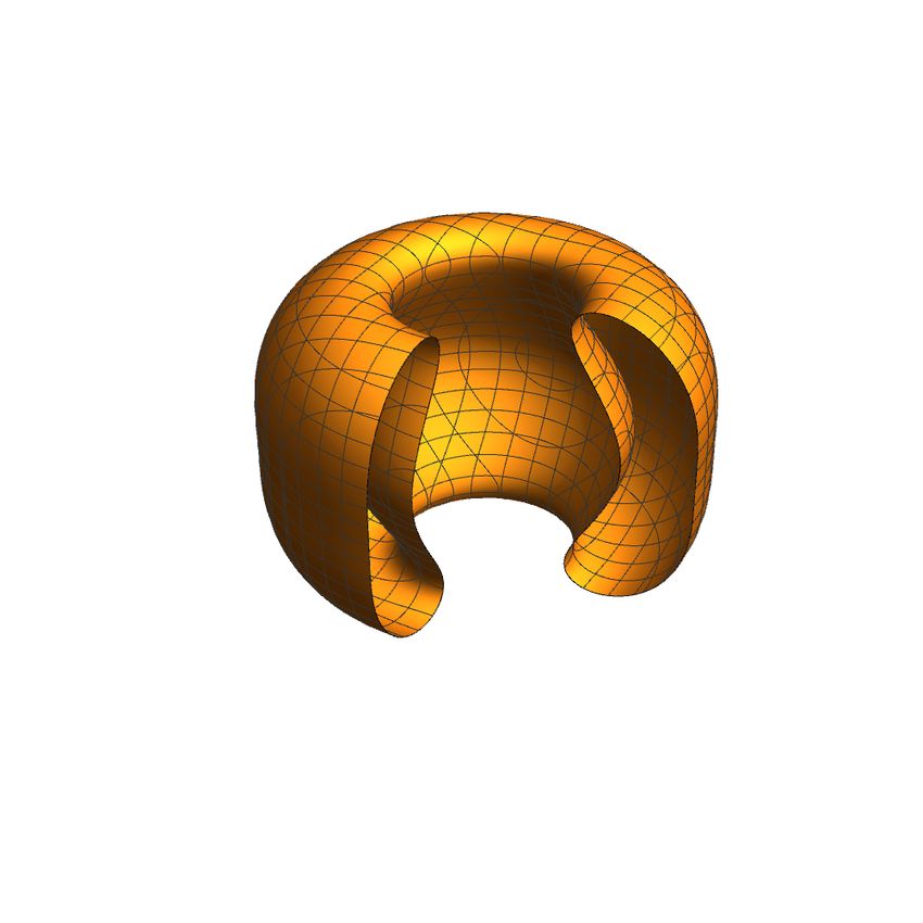
2

features. For instance, they may possess disjunct ergo-regions consisting of an ergo-sphere
surrounded by an ergo-torus (i.e., a so-called “ergo-Saturn”) [5, 11].
    The family of rotating hairy BHs with synchronised hair is characterized both by the
usual set of physical quantities like mass, angular momentum and Noether charge, as well as
by two integers: the azimuthal winding number of the complex scalar field n, often referred
to as its rotational quantum number, and its node number k. Most of the studies have
focused on the nodeless fundamental solutions with n = 1 and k = 0. Only recently also
radially and angularly excited hairy BHs with k 6= 0 [20], and rotationally excited hairy BHs
with n > 1 were considered in [21] (see also the case of scalarized hairy BHs [11]).
    By analogy with axially-symmetric spinning Q-balls in flat space [27–32], as well as
based the existence of the corresponding perturbative Q-cloud solutions [8, 9], for each
value of integer winding number n, there should be two types of spinning solutions possessing
different parity, so called parity-even and parity-odd rotating hairy BHs.
    So far, however, only parity-even rotating hairy BHs were investigated in detail, whereas
the parity-odd rotating hairy BHs received little attention [20]. In this letter we construct a
large set of axially symmetric stationary parity-odd hairy BHs in the massive complex Klein-
Gordon theory minimally coupled to Einstein’s gravity and discuss their physical properties.
    We show that a distinctive new feature of the parity-odd hairy BH solutions is related
to the shapes of their ergo-regions, which, may represent an ergo-sphere, an ergo-Saturn,
or a new type of composite ergo-surface, representing an ergo-double-torus-Saturn, where
an ergo-sphere is surrounded by two ergo-tori located symmetrically with respect to the
equatorial plane.

                                    II.   THE MODEL

   We consider the Einstein-Klein-Gordon model, that is the theory of a single non self-
interacting massive complex scalar field φ, which is minimally coupled to Einstein gravity
in an asymptotically flat 3+1 dimensional space-time. The action of the model is
                                      √
                                  Z
                                              R
                              S=        −g       − Lm d4 x,                            (1)
                                             4α2

where R is the Ricci scalar curvature with respect to the Einstein metric gµν , g is the
determinant of the metric tensor, α2 = 4πG is the gravitational coupling constant with
Newton’s constant G, and Lm is the matter field Lagrangian

                                    Lm = |∂µ φ|2 + µ2 |φ|2 ,                               (2)

where µ is the mass of scalar field.
   The action (1) is invariant with respect to global U(1) transformations of the complex
scalar field, φ → φeiχ , where χ is a constant. Associated with this symmetry is the Noether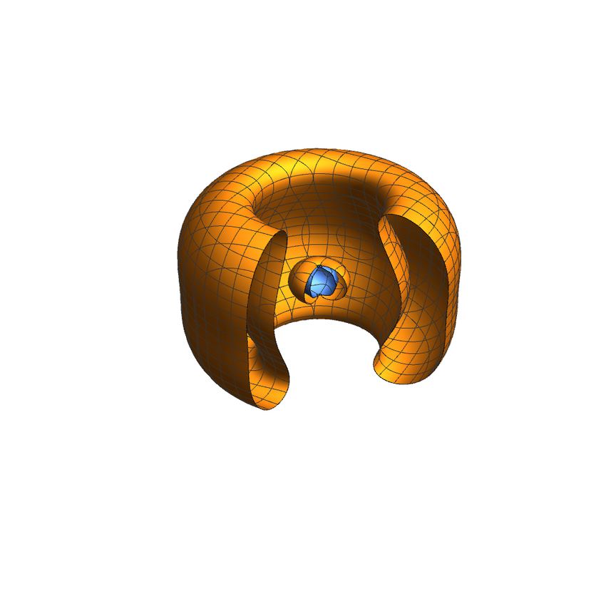
3

4-current
                                 jµ = i(φ∂µ φ∗ − φ∗ ∂µ φ) ,                              (3)
                                                R√
and the corresponding conserved charge is Q =       −gj t d3 x.
  Variation of the action (1) with respect to the metric leads to the Einstein equations
                                             1
                                        Rµν − Rgµν = 2α2 Tµν ,                                           (4)
                                             2
where
                                Tµν = (∂µ φ∂ν φ∗ + ∂ν φ∂µ φ∗ ) − Lm gµν ,                                (5)
is the stress-energy tensor of the scalar field.
    The corresponding equation of motion for the scalar field is the linear Klein-Gordon
equation
                                          − µ2 φ = 0 ,

                                                                                      (6)
where  represents the covariant d’Alembert operator. It should be noted that, both param-
eters of the model (1), α and µ, can be rescaled away via transformations of the coordinates
                      µ
and the field, xµ → xµ and φ → αφ . In the numerical calculations we fix these parameters to
α = 0.5 and µ = 1.

                         A.    Spinning axially-symmetric configurations

   To obtain stationary spinning axially-symmetric field configurations, we take into account
the presence of two commuting Killing vector fields ξ = ∂t and η = ∂ϕ , where t and ϕ are
the time and azimuthal coordinates, respectively. In these coordinates the metric can be
written in Lewis-Papapetrou form
                                                                         2
                 2          2        2     2 2
                                                  2    2            W
               ds = −F0 dt + F1 dr + r dθ + r sin θF2 dϕ − dt ,                           (7)
                                                                      r

where the four metric functions F0 , F1 , F2 and W depend on r and θ only.
  The axially-symmetric ansatz for the stationary scalar field is

                                          φ = f (r, θ)ei(ωt+nϕ) ,                                        (8)

where ω is the frequency of field, and n ∈ Z is the azimuthal winding number 1 .
  By substituting the ansatz (8) into the field equation (6), we obtain

                 √ ∂f                       √ ∂f

   1 ∂        rr               1 ∂       θθ
                                                     − n2 g ϕϕ − 2g ϕt + ω 2 g tt f = µ2 f . (9)

 √          g     −g      +√           g     −g
   −g ∂r             ∂r        −g ∂θ            ∂θ

1
    Note that we are using the rescaled dimensionless frequency ω → ω/µ in the numerical calculations.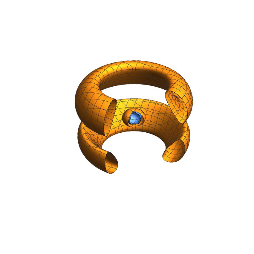
4

This implies in the case of the Kerr background, that the variables separate, f (r, θ) =
Rln (r)Sln (θ), where Sln are the spheroidal harmonics, −l ≤ n ≤ l and Rln (r) the radial
functions [1, 3]. A linear analysis of the spatial asymptotic behavior of the field, where the
metric
  √ functions approach the flat space limit, shows that the scalar field is proportional to
 − µ2 −ω 2 r
e            , thus for ω < µ the scalar field is exponentially localized.
   The structure of the dynamical equation (9) suggests that, analogous to the case of the
spinning axially-symmetric Q-balls and boson stars [27–32], the hairy BH solutions of the
Einstein-Klein-Gordon system may also be either symmetric with respect to reflections in
the equatorial plane, θ → π − θ, or antisymmetric, as conjectured in [9]. The solutions of
the first type are referred to as parity-even, while the configurations of the second type are
termed parity-odd. While previous studies of rotating hairy BHs focused entirely on the
case of parity-even solutions, see e.g. [7–21], in this paper we shall construct and discuss
parity-odd solutions.
   We assume the existence of a rotating event horizon, located at a constant value of radial
variable r = rh > 0. The Killing vector of the horizon is the helicoidal vector field

                                              χ = ξ + Ωh η ,                                 (10)

where the horizon angular velocity is fixed by the value of the metric function W on the
horizon
                                        gφt
                               Ωh = −            =W       .
                                        gtt r=rh     r=rh

The presence of a rotating horizon allows for the formation of stationary scalar clouds,
supported by the synchronisation condition [3–6]

                                                    ω = nΩh                                  (11)

between the event horizon angular velocity Ωh , the scalar field frequency ω, and the winding
number n. This condition implies that there is no flux of scalar field into the black hole
[3–6].
   It is convenient to make use of the exponential parametrization of the metric fields
                              2
                      1 − rrh      f0
                                                  rh 4 f1           rh 4 f2
               F0 =            2 e    , F1 =   1 +      e   F 2 =  1 +      e .          (12)
                      1 + rh                       r                   r

                            r

Then a power series expansion near the horizon yields the conditions of regularity of the
profile function f and the metric functions fi

                     ∂r f   r=rh
                                   = ∂r f0   r=rh
                                                    = ∂r f1   r=rh
                                                                     = ∂r f2   r=rh
                                                                                      = 0.   (13)

These boundary conditions supplement the synchronization condition (11) imposed on the
metric function W .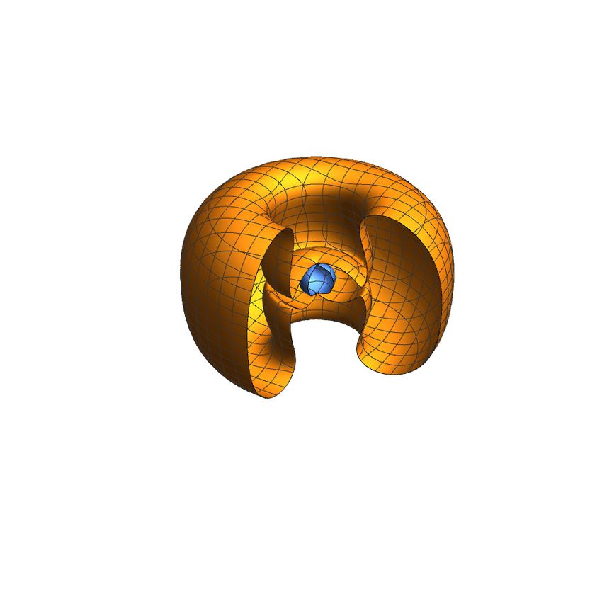
5

  The requirement of asymptotic flatness at spatial infinity yields

                  f0   r→∞
                              = f1        r→∞
                                                = f2   r→∞
                                                               =W       r→∞
                                                                               = 0,     f      r→∞
                                                                                                     = 0.      (14)

Axial symmetry and regularity impose the following boundary conditions on the symmetry
axis at θ = 0, π

              f   θ=0,π
                          = ∂θ f0     θ=0,π
                                                = ∂θ f1     θ=0,π
                                                                    = ∂θ f2   θ=0,π
                                                                                      = ∂θ W    θ=0,π
                                                                                                        = 0.   (15)

The symmetry of the solutions with respect to the reflections in the equatorial plane allows
us to consider the range of values of the angular variable θ ∈ [0, π/2]. The corresponding
boundary conditions are

                          ∂θ f0   θ= π2
                                          = ∂θ f1   θ= π2
                                                            = ∂θ f2   θ= π2
                                                                              = ∂θ W   θ= π2
                                                                                               = 0,            (16)

and for the parity-even solutions ∂θ f θ= π = 0, while for parity-odd solutions f θ= π = 0.
                                          2                                          2
  Note that the condition of  the absenceof a conical singularity requires that the deficit
angle should vanish, δ = 2π 1 − lim FF21 = 0. Hence the solutions should satisfy the
                                                 θ→0
constraint F2 θ=0 = F1 θ=0 . In our numerical scheme we explicitly verified (within the
numerical accuracy) this condition on the symmetry axis.
   Asymptotic expansions of the metric functions at the horizon and at spatial infinity
yield important physical properties of the BHs. The total ADM mass M and the angular
momentum J of the spinning hairy BHs can be read off from the asymptotic subleading
behaviour of the metric functions as r → ∞
                           α2 M                    α2 J

                                        1                   2      1
                gtt = −1 +       + O 2 , gϕt =           sin θ + O 2 .             (17)
                            πr          r           πr             r
   The ADM charges can be represented as sums of the contributions from the event horizon
and the scalar hair: M = Mh + MΦ and J = Jh + JΦ , respectively. These contributions can
be evaluated separately from Komar integrals
                        I                       I
                     1                        1
          Mh = − 2 dSµν ∇ ξ , Jh = 2 dSµν ∇µ η ν ,
                                 µ ν
                   2α S                      4α S
                       Z                              Z                            (18)
                    1            µ ν      µ        1             µ ν   1 µ
          MΦ = − 2        dSµ (2Tν ξ − T ξ ), JΦ = 2     dSµ Tν η − T η ,
                   α V                            2α V                 2
where S is the horizon 2-sphere and V denotes an asymptotically flat spacelike hypersurface
bounded by the horizon.
   Note that, analogous to the angular momentum of the stationary rotating boson stars,
there is the quantization relation for the angular momentum of the scalar field, JΦ = nQ,
where Q is the Noether charge and n is the winding number of the scalar field.
   The horizon properties include the Hawking temperature Th , which is is proportional to
the surface gravity κ2 = − 21 ∇µ χν ∇µ χν ,
                                  κ         1    h                i
                          Th =       =        exp (f0 − f1 ) r=r ,                     (19)
                                 2π     16πrh                   h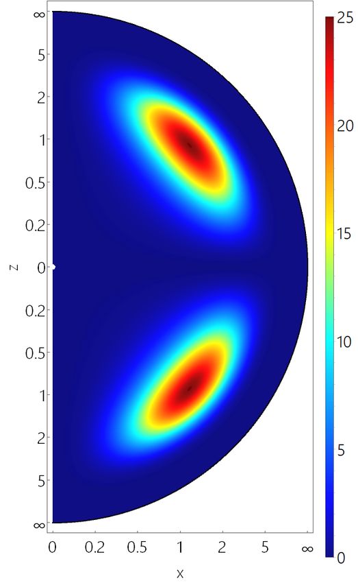
6

where χ is the horizon Killing vector (10). Another property of considerable interest is the
horizon area Ah , given by
                                    Z π             h              i
                                  2
                        Ah = 32πrh      dθ sin θ exp (f1 + f2 ) r=r .                   (20)
                                                                               h
                                             0

The rotating hairy BHs satisfy the Smarr relation [4–6]

                                        M = 2Th S + 2Ωh Jh + MΦ ,                                          (21)

where S = απ2 Ah is the entropy of the black hole and MΦ is the scalar field energy outside
the event horizon (18). The hairy black holes also satisfy the first law of thermodynamics
[4–6]
                                   dM = Th dS + Ωh dJ .

                                    III.   NUMERICAL RESULTS

    We have solved the boundary value problem for the coupled system of nonlinear partial
differential equations (4) and (6) with boundary conditions (13)-(15) using a fourth-order
finite difference scheme. The system of equations is discretized on a grid with 101 × 101
points. We have introduced the new radial coordinate x = r−r       h
                                                                 r+c
                                                                     , which maps the semi-
infinite region [0, ∞) onto the unit interval [0, 1]. Here c is an arbitrary constant which
is used to adjust the contraction of the grid. The emerging system of nonlinear algebraic
equations is solved using a modified Newton method. The underlying linear system is solved
with the Intel MKL PARDISO sparse direct solver. The errors are on the order of 10−9 . All
calculations have been performed using the CESDSOL 2 library.
    Let us now briefly summarize the key results we have obtained by solving the field equa-
tions of the model (1) with the boundary conditions discussed above, focusing our study on
the n = 1 parity-odd hairy BH solutions. We recall that such hairy BHs exist only for n > 0.
The only spherically symmetric solutions with n = 0 are globally regular boson stars.
    First, we observe that parity-odd n = 1 solutions exist in the regular limit rh = 0.
They represent a new family of mini boson stars, which do not possess a flat space limit.
The dependence of these solutions on the frequency ω is qualitatively similar to that of
the spinning boson stars, that can be linked to flat space Q-balls because of the presence
of higher order self-interaction terms, and other gravitating solitons [11, 19, 27–31]. The
existence region of the spinning axially symmetric solutions is limited by ωmax = µ from
above and some ωmin > 0 from below.

2
    Complex Equations – Simple Domain partial differential equations SOLver is a C++ library being devel-
    oped by IP. It provides tools for the discretization of an arbitrary number of arbitrary nonlinear equations
    with arbitrary boundary conditions on direct product arbitrary dimensional grids with arbitrary order of
    accuracy.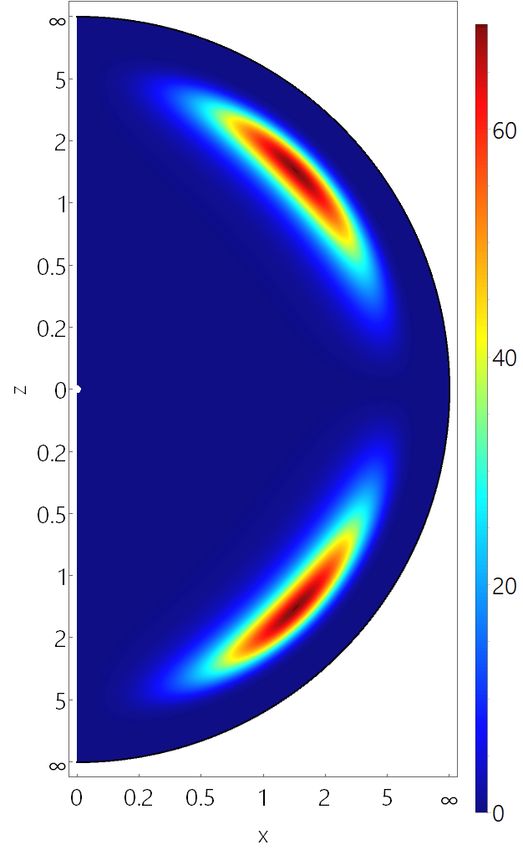
7
100
90
r =0.03 r =0.04 r =0.06
h
h r =0.05 h
h
80
r =0.06 30
h
70
r =0
25 h
60
20
55
M
50
M
r =0.01 15
h
40
r =0 r =0.02
h h 50
10
30
5
45
20
Kerr
0
0,980 0,985 0,990 0,995 1,000
10
40
25 30 35 40
0
0 10 20 30 40 50 60 70 80 90 100
2
/ J
2 6
r =0.05
h
r =0.04
h
4
01
0.
= r =0.03
r h h
1
2
0.0 2 r =0.06
r = h
h
2
T /
Ah/
0.5
H
.03
r =0
h
1
0.5
r =0.06
h
0.1 r =0.02
h
r =0.04 0.1
h
r =0.01
0.01 r =0.05 h
h
0.01
0 0
0,65 0,70 0,75 0,80 0,85 0,90 0,95 1,00 0,65 0,70 0,75 0,80 0,85 0,90 0,95 1,00
/ /
0.02 1,0
r =0.05
h
r =0.01
0.01 h
0,9
r =0.06
h
r =0.02
h
0,8
(r )
r =0.04
h
e
h
r =0.05
L /L
h
0,7
max
r =
p
0.001 h 0.0
3
f
0,6
r =0.02
h
r =0.03 r =0.06
h
h
0,5 r =0.01
h
r =0.04
h
0 0,4
0,65 0,70 0,75 0,80 0,85 0,90 0,95 1,00 0,65 0,70 0,75 0,80 0,85 0,90 0,95 1,00
/ /
FIG. 1: Properties of parity-odd n = 1 boson stars and hairy BHs: ADM mass M vs frequency ω,
where the shaded area corresponds to the domain of existence of vacuum Kerr BHs (upper left),
ADM mass M vs angular momentum J (upper right), Hawking temperature Th vs frequency ω
(middle left), horizon area Ah vs frequency ω (middle right), maximal value of the scalar field on
Lp
the event horizon fmax (rh ) vs frequency ω (lower left), and the horizon deformation = Le in
terms of the ratio of the polar and equatorial circumferences vs frequency ω (lower right), for a set
of values of the horizon radius parameter rh .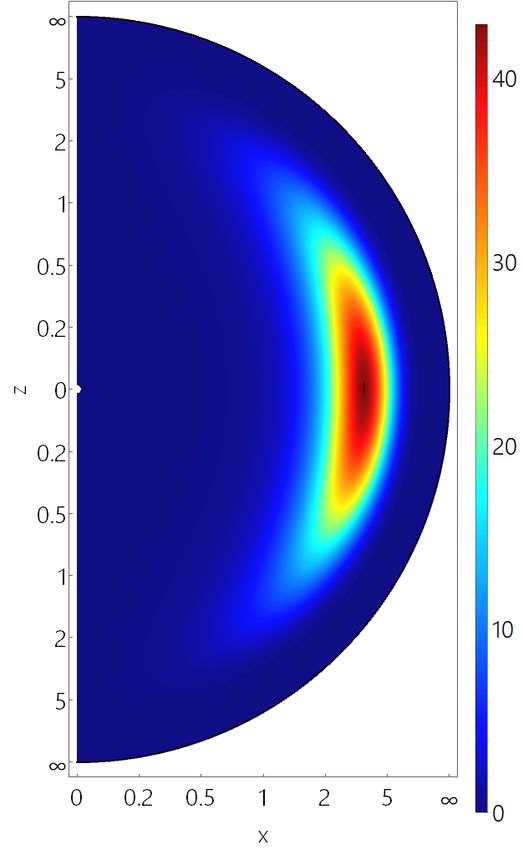
8

                                                                   odd-parity

                M

                             even-parity

                                             Kerr

                                                    /

FIG. 2: Comparison of parity-odd and parity-even n = 1 boson stars and hairy BHs: ADM mass
M vs frequency ω for horizon radius parameter rh = 0 and rh = 0.01. The shaded area corresponds
to the domain of existence of vacuum Kerr BHs.

   The dependence of the ADM mass and the Noether charge of the parity-odd n = 1
regular rh = 0 configurations on the angular frequency both exhibit a typical inspiralling
pattern, as shown in Fig. 1, left upper plot, for the mass. As the frequency ω decreases from
ωmax , the mass M gradually increases approaching its maximum at some critical value of the
frequency ωM . From that point onwards the mass of the solutions on the first fundamental
branch decreases until the minimum frequency ωmin is reached. At ωmin the fundamental
forward branch backbends into a second (backward) branch. A third (forward) branch and a
fourth (backward) branch are also visible in Fig. 1, upper plot, forming the first few branches
of a spiral. We note the consistency of this figure with the one presented in [20], where,
however, no further properties of these hairy BHs were discussed.
   In Fig. 1, middle left plot, we show the mass M of the regular parity-odd solutions
versus the total angular momentum J. As seen in the figure, multiple cusps occur in the
curves as the branches bifurcate at the respective maximal and minimal values of the mass.
As expected, for the same set of values of the parameters of the model, the mass of the
parity-odd configurations is higher than the mass of the parity-even solutions, and the
corresponding value of the minimal frequency ωmin of the parity-odd configurations is higher,
as demonstrated in Fig. 2.
9 FIG. 3: Stress-energy tensor component ρ = −Ttt of n = 1 hairy BHs in the y = 0 plane for parity- even (left column) and parity-odd (right column) solutions with frequency ω = 0.8 and horizon radius parameter rh = 0.01 on the fundamental forward branch (upper row) and on the backward branch (lower row).
10

   The domain of existence of parity-odd hairy BHs is scanned by varying the frequency ω,
and the horizon radius parameter rh . In Fig. 1, upper plot, we illustrate the dependence of
the ADM mass of the spinning hairy BHs on the frequency ω for a set of values of rh . As
the size of the horizon is increased from zero, the hairy BHs emerge from the corresponding
regular solutions. When the angular frequency decreases from ωmax = 1, the mass of the
upper branch solutions increases, approaching a maximum at some value of frequency ωM .
As rh increases, the value of the maximal mass decreases. The further dependence on the
frequency then depends on the value of rh .
   For small values of rh the spiralling type of the critical behaviour is changed to a multi-
branch structure with a smaller number of branches. The last branch then dives into the
region, where the Kerr BHs reside. Here it merges at some frequency ωend < µ with the
existence line for the parity-odd scalar clouds around Kerr BHs. In this limit the scalar field
trivializes, and the branch ends on the respective Kerr BH. This behaviour is qualitatively
similar to the one observed for parity-even hairy BHs with synchronised hair [1, 4, 6] and
also to the one observed in similar models [19].
   As rh increases further, the multi-branch structure is replaced with a two-branch scenario,
with the first (upper, forward) branch connected to the perturbative excitations at ωmax = µ
and the second (lower, backward) branch, terminating at the respective Kerr solution as
ω → ωend . The minimum angular frequency ωmin increases as rh increases. At some point the
critical frequency ωM , which corresponds to the maximal value of the ADM mass, becomes
the minimal allowed frequency ωmin . The maximum value of the frequency along the second
branch ωend is slowly increasing and approaches ωmax = 1 as the loop shrinks to zero.
   Turning to the horizon properties, we note that the Hawking temperature decreases along
the constant rh curves, as shown in Fig. 1, middle right plot. The larger rh , the lower is the
temperature on the fundamental branches of these hairy BHs. For the smaller values of rh the
value of the scalar field on the horizon f (rh ) increases both along the fundamental forward
branch and along the second backward branch, while it decreases when the configuration
approaches the Kerr limit, as seen in Fig. 1, lower left plot. For the higher values of rh , where
the critical frequency ωM ∼ ωmin , the value of f (rh ) increases along the forward branch, and
decreases along the backward branch.
   To illustrate the different scalar field distributions for the parity-even and parity-odd
n = 1 solutions, we exhibit in Fig. 3 the stress-energy component ρ = −Ttt for both parity
cases for the same parameters rh = 0.01 and ω = 0.8, with one set of solutions on the first
(forward) branch and another on the second (backward) branch. Clearly, for the parity-even
solutions the matter distribution is of the typical toroidal shape, whereas for the parity-odd
solutions it possesses the double-torus structure. On the second (backward) branch the
solutions become more compact.
   Let us next consider the geometry of the ergo-surfaces of the parity-odd spinning BHs,
11
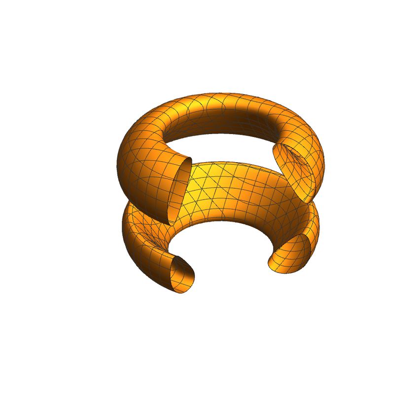
FIG. 4: Ergosurfaces of parity-odd n = 1 boson stars with frequency ω = 0.75 (left) and ω = 0.8
(right) on the backward branch.
defined as the zero locus of the normalized time-like Killing vector ξ · ξ = 0, or
gtt = −F0 + sin2 θF2 W 2 = 0 . (22)
The presence of ergo-regions in rotating boson stars was realized and investigated in [28, 34],
where the non-trivial topology of the ergo-regions was discussed. For the spinning boson
stars ergo-regions appear typically on the fundamental branch in the vicinity of the maximal
mass, where the angular frequency ω decreases below ωM [5, 28]. The topology of the ergo-
region of the spinning regular parity-even solutions is an ergo-torus, S 1 × S 1 . Interestingly,
for the spinning regular parity-odd solutions also ergo-double-tori, (S 1 × S 1 ) (S 1 × S 1 ),
L
arise [28], as illustrated in Fig. 4.
The hairy BHs, on the other hand, can either feature a Kerr-like S 2 ergo-region, or an
“ergo-Saturn”, with topology S 2 (S 1 × S 1 ), when they possess parity-even scalar hair [5].
L
For the parity-odd hairy BHs, again Kerr-like ergo-surfaces with S 2 topology are present on
the fundamental branch, as shown in Fig. 5, left plot. However, on the secondary branches
this changes, and ergo–double-tori appear in addition to the S 2 ergo-sphere. Thus a new type
of ergosurface topology arises, representing an ergo-double-torus-Saturn (S 1 × S 1 ) (S 1 ×
L
S 1 ) S 2 , illustrated in Fig. 5, second plot. Moving on along the branches of constant
L
rh , we observe that the ergo-double-tori merge into single deformed ergo-tori, and, as the
configurations approach the Kerr limit, into a single ergo-sphere S 2 , shown in Fig. 5, right
plot.
We have also studied the parity-odd solutions with higher values of the winding number
n > 1, shown in Fig. 6. Generally, the branch structure of these solutions is similar to what12
FIG. 5: Ergosurfaces of parity-odd n = 1 hairy BHs with horizon radius parameter rh = 0.01 and
frequencies ω = 0.75 (1), ω = 0.8 (2), ω = 0.85 (3) and ω = 0.93 (4) on the backward branch. Blue
surfaces represent the horizon.
we observed for the n = 1 hairy BHs, however, their masses are higher and they exist within
a larger frequency interval.
IV. CONCLUSIONS
We have considered rotating hairy BHs in Einstein-Klein-Gordon theory, constructing for
the first time BHs with parity-odd scalar hair. Analogous to their parity-even counterparts,13
0.5
n=4
0.25
TH/
M
0.1
n=3
n=2 n=1
n=1
n= 3 n= 2
0.01 n= 4
Kerr
0
0,6 0,7 0,8 0,9 1,0
/ /
FIG. 6: Properties of parity-odd n ≥ 1 hairy BHs: ADM mass M vs frequency ω (left), Hawking
temperature Th vs frequency ω (right), for the horizon radius parameter rh = 0.05. The shaded
area corresponds to the domain of existence of vacuum Kerr BHs.
these solutions emerge from the corresponding parity-odd boson star solutions, when a small
finite event horizon radius is imposed via the boundary conditions. Their domain of existence
is then determined by the regular boson star solutions on the one hand and the Kerr BHs
on the other hand, where they merge with the existence line for the parity-odd scalar clouds
around Kerr BHs. In fact, many of the properties of these parity-odd hairy BHs are similar
to those of their parity-even counterparts.
However, the parity-odd scalar field also leads to new features. Thus the scalar field
around the BHs is often concentrated in two tori, located symmetrically with respect to the
equatorial plane. Consequently the energy density is no longer centered in the equatorial
plane. A further consequence of this distribution of the energy density is the occurrence
of a new type of ergo-surface topology. Indeed, these rotating hairy BHs may feature an
ergo-double-torus-Saturn (S 1 × S 1 ) (S 1 × S 1 ) S 2 .
L L
We expect analogous parity-odd hairy BHs to be present in numerous other cases,
where parity-even BHs have been reported. One particular model, where they arise, is the
Friedberg-Lee-Sirling model coupled to Einstein gravity. These solutions and their properties
will be reported elsewhere [33].
Acknowledgements– We are grateful to Burkhard Kleihaus and Eugen Radu for inspir-
ing and valuable discussions. This work was supported in part by the DFG Research Training
Group 1620 Models of Gravity as well as by and the COST Action CA16104 GWverse. Ya.S.
gratefully acknowledges the support of the Alexander von Humboldt Foundation and from
the Ministry of Education and Science of Russian Federation, project No 3.1386.2017. I.P.14
would like to acknowledge support by the DAAD Ostpartnerschaft Programm.
[1] C. A. R. Herdeiro and E. Radu, Int. J. Mod. Phys. D 24 (2015) no.09, 1542014
[2] M. S. Volkov, arXiv:1601.08230 [gr-qc].
[3] S. Hod, Phys. Rev. D 86 (2012) 104026 Erratum: [Phys. Rev. D 86 (2012) 129902]
[4] C. A. R. Herdeiro and E. Radu, Phys. Rev. Lett. 112 (2014) 221101
[5] C. Herdeiro and E. Radu, Phys. Rev. D 89 (2014) no.12, 124018
[6] C. Herdeiro and E. Radu, Class. Quant. Grav. 32 (2015) no.14, 144001
[7] S. Hod, Phys. Rev. D 90 (2014) no.2, 024051
[8] C. L. Benone, L. C. B. Crispino, C. Herdeiro and E. Radu, Phys. Rev. D 90, no. 10, 104024
(2014)
[9] C. Herdeiro, E. Radu and H. Runarsson, Phys. Lett. B 739 (2014) 302
[10] C. A. R. Herdeiro and E. Radu, Int. J. Mod. Phys. D 23 (2014) no.12, 1442014
[11] B. Kleihaus, J. Kunz and S. Yazadjiev, Phys. Lett. B 744 (2015) 406
[12] C. A. R. Herdeiro, E. Radu and H. Runarsson, Phys. Rev. D 92 (2015) no.8, 084059
[13] C. Herdeiro, J. Kunz, E. Radu and B. Subagyo, Phys. Lett. B 748, 30 (2015)
[14] C. Herdeiro, E. Radu and H. Runarsson, Class. Quant. Grav. 33 (2016) no.15, 154001
[15] Y. Brihaye, C. Herdeiro and E. Radu, Phys. Lett. B 760 (2016) 279
[16] S. Hod, Phys. Lett. B 751 (2015) 177
[17] C. Herdeiro, J. Kunz, E. Radu and B. Subagyo, Phys. Lett. B 779, 151 (2018)
[18] C. Herdeiro, I. Perapechka, E. Radu and Y. Shnir, JHEP 1810 (2018) 119
[19] C. Herdeiro, I. Perapechka, E. Radu and Y. Shnir, JHEP 1902 (2019) 111
[20] Y. Q. Wang, Y. X. Liu and S. W. Wei, Phys. Rev. D 99 (2019) no.6, 064036
[21] J. F. M. Delgado, C. A. R. Herdeiro and E. Radu, arXiv:1903.01488 [gr-qc].
[22] W. E. East and F. Pretorius, Phys. Rev. Lett. 119 (2017) no.4, 041101
[23] C. A. R. Herdeiro and E. Radu, Phys. Rev. Lett. 119 (2017) no.26, 261101
[24] F. E. Schunck and E. W. Mielke, Phys. Lett. A 249, 389 (1998).
[25] F. D. Ryan, Phys. Rev. D 55, 6081 (1997).
[26] S. Yoshida and Y. Eriguchi, Phys. Rev. D 56, 762 (1997).
[27] B. Kleihaus, J. Kunz and M. List, Phys. Rev. D 72 (2005) 064002 .
[28] B. Kleihaus, J. Kunz, M. List and I. Schaffer, Phys. Rev. D 77 (2008) 064025
[29] M.S. Volkov and E. Wohnert, Phys. Rev. D 66 (2002) 085003.
[30] E. Radu and M.S. Volkov, Phys. Rept. 468 (2008) 101.
[31] J. Kunz, E. Radu and B. Subagyo, Phys. Rev. D 87 (2013) no.10, 104022
[32] V. Loiko, I. Perapechka and Y. Shnir, Phys. Rev. D 98 (2018) no.4, 045018
[33] J. Kunz, I. Perapechka and Y. Shnir, in preparation
[34] V. Cardoso, P. Pani, M. Cadoni and M. Cavaglia, Phys. Rev. D 77, 124044 (2008)You can also read