Exposing Digital Forgeries from JPEG Ghosts
←
→
Page content transcription
If your browser does not render page correctly, please read the page content below
1

        Exposing Digital Forgeries from JPEG Ghosts
                                                      Hany Farid, Member, IEEE

   Abstract— When creating a digital forgery, it is often necessary      the underlying DCT coefficients is both computationally non-
to combine several images, for example, when compositing one             trivial, and prone to some estimation error, which leads to vul-
person’s head onto another person’s body. If these images were           nerabilities in the forensic analysis. In comparison to [13], our
originally of different JPEG compression quality, then the digital
composite may contain a trace of the original compression                approach does not require that the image be cropped in order
qualities. To this end, we describe a technique to detect if part        to detect blocking inconsistencies. In addition, our approach
of an image was initially compressed at a lower quality than the         can detect local tampering unlike the global approach of [13]
rest of the image. This approach is applicable to images of high         which can only detect an overall crop and re-compression.
and low quality and resolution.                                          And in comparison to [14], our approach, although likely
  Index Terms— Digital Forensics, Digital Tampering                      not as powerful, is computationally much simpler and does
                                                                         not require a large database of images to train a support
                                                                         vector machine. As with all forensic analysis, each of these
                        I. I NTRODUCTION                                 techniques have their relative benefits and drawbacks. The
   Recent advances in digital forensics have given rise to               new technique described here contributes to the growing set
many techniques for detecting photographic tampering. These              forensic analysis tools based on JPEG artifacts, and should
include techniques for detecting cloning [1], [2]; splicing [3];         prove useful as a new tool in the arsenal of forensic analysts.
re-sampling artifacts [4], [5] ; color filter array aberrations [6];
disturbances of a camera’s sensor noise pattern [7]; chromatic                                 II. JPEG G HOSTS
aberrations [8]; and lighting inconsistencies [9], [10], [11].              In the standard JPEG compression scheme [16], [17], a color
Although highly effective in some situations, many of these              image (RGB) is first converted into luminance/chrominance
techniques are only applicable to relatively high quality im-            space (YCbCr). The two chrominance channels (CbCr) are
ages. A forensic analyst, however, is often confronted with low          typically subsampled by a factor of two relative to the lumi-
quality images, in terms of resolution and/or compression. As            nance channel (Y). Each channel is then partitioned into 8 × 8
such there is a need for forensic tools that are specifically            pixel blocks. These values are converted from unsigned to
applicable to detecting tampering in low quality images. This            signed integers (e.g., from [0, 255] to [−128, 127]). Each block
is particularly challenging since low quality images often               is converted to frequency space using a 2-D discrete cosine
destroy any statistical artifacts that could be used to detect           transform (DCT). Each DCT coefficient, c, is then quantized
tampering.                                                               by an amount q:
   Along these lines, Ye, et. al developed a technique to
estimate the local JPEG compression blocking artifacts [12]                                    ĉ = round(c/q),                       (1)
– inconsistencies in these artifacts were then used as evidence
of tampering. Luo, et. al developed a technique to detect                where the quantization q depends on the spatial frequency and
inconsistencies in JPEG blocking artifacts that arise from               channel. Larger quantization values q yield better compression
mis-alignments of JPEG blocks relative to their original lat-            at the cost of image degradation. Quantization values are
tice [13]. And, He et. al developed a technique to detect local          typically larger in the chrominance channels, and in the higher
traces of double JPEG compression [14] (this work expands                spatial frequencies, roughly modeling the sensitivity of the
on a global approach to detecting double compression [15]).              human visual system.
   A complementary approach to detecting tampering in low                   Consider now a set of coefficients c1 quantized by an
quality images is presented here. This approach detects tam-             amount q1 , which are subsequently quantized a second time
pering which results when part of a JPEG image is inserted               by an amount q2 to yield coefficients c2 . With the exception
into another higher quality JPEG image. For example, when                of q2 = 1 (i.e., no quantization), the difference between c1
one person’s head is spliced onto another person’s body,                 and c2 will be minimal when q2 = q1 . It is obvious that
or when two separately photographed people are combined                  the difference between c1 and c2 increases for quantization
into a single composite. This approach works by explicitly               value q2 > q1 since the coefficients become increasingly more
determining if part of an image was originally compressed at             sparse as q2 increases. For values of q2 < q1 , the difference
a lower quality relative to the rest of the image.                       between c1 and c2 also increases because although the second
   In comparison to [12], our approach does not require an               quantization does not affect the granularity of the coefficients,
estimate of the DCT quantization from an assumed original                it does cause a shift in their values. Shown in Fig. 1(a), for
part of the image. Estimating the quantization from only                 example, is the sum of squared differences between c1 and c2
                                                                         as a function of the second quantization q2 , where q1 = 17, and
  H. Farid (farid@cs.dartmouth.edu) is with the Department of Computer   where the coefficients c1 are drawn from a normal zero-mean
Science at Dartmouth College, 6211 Sudikoff Lab, Hanover NH 03755.       distribution. Note that this difference increases as a function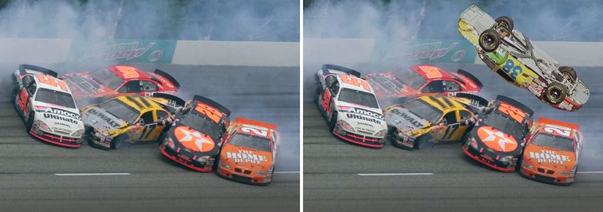
2

of increasing q2 , with the exception of q2 = q1 , where the                   These fluctuations are due to the underlying image content.
difference is minimal. If q1 is not prime, as in our example,                  Specifically, because the image difference is computed across
then multiple minima may appear at quality values q2 that                      all spatial frequencies, a region with small amounts of high
are integer multiples of q1 . As will be seen below, this issue                spatial frequency content (e.g., a mostly uniform sky) will have
can be circumvented by averaging over all of the JPEG DCT                      a lower difference as compared to a highly textured region
coefficients.                                                                  (e.g., grass). In order to compensate for these differences,
   Consider now a set of coefficients c0 quantized by an                       we consider a spatially averaged and normalized difference
amount q0 , followed by quantization by an amount q1 < q0 to                   measure. The difference image is first averaged across a b × b
yield c1 . Further quantizing c1 by q2 yields the coefficients c2 .            pixel region:
As before, the difference between c1 and c2 will be minimal                                               3     b−1 b−1
when q2 = q1 . But, since the coefficients were initially                                              1X 1 X X
                                                                                  δ(x, y, q)   =                        [f (x + bx , y + by , i)
quantized by q0 , where q0 > q1 , we expect to find a second                                           3 i=1 b2
                                                                                                                 bx =0 by =0
minimum when q2 = q0 . Shown in Fig. 1(b) is the sum
                                                                                                          −fq (x + bx , y + by , i)]2 ,            (3)
of squared differences between c1 and c2 , as a function of
q2 , where q0 = 23 and q1 = 17. As before, this difference                     and then normalized so that the averaged difference at each
increases as a function of increasing q2 , reaches a minimum                   location (x, y) is scaled into the range [0, 1]:
at q2 = q1 = 17, and most interestingly has a second local
                                                                                                      δ(x, y, q) − minq [δ(x, y, q)]
minimum at q2 = q0 = 23. We refer to this second minimum                           d(x, y, q) =                                           .        (4)
as a JPEG ghost, as it reveals that the coefficients were                                           maxq [δ(x, y, q)] − minq [δ(x, y, q)]
previously quantized (compressed) with a larger quantization                      Although the JPEG ghosts are often visually highly salient,
(lower quality).                                                               it is still useful to quantify if a specified region is statistically
   Recall that the JPEG compression scheme separately quan-                    distinct from the rest of the image. To this end, the two-sample
tizes each spatial frequency within a 8 × 8 pixel block. One                   Kolmogorov-Smirnov statistic [18] is employed to determine
approach to detecting JPEG ghosts would be to separately                       if the distribution of differences, Equation(4), in two regions
consider each spatial frequency in each of the three lumi-                     are similar or distinct. The K-S statistic is defined as:
nance/color channels. However, recall that multiple minima are
possible when comparing integer multiple quantization values.                                   k     =    max |C1 (u) − C2 (u)|,                  (5)
                                                                                                             u
If, on the other hand, we consider the cumulative effect of
                                                                               where C1 (u) and C2 (u) are the cumulative probability distri-
quantization on the underlying pixel values, then this issue is
                                                                               butions of two specified regions in the computed difference
far less likely to arise (unless all 192 quantization values at
                                                                               d(x, y, q), where each value of q is considered separately.
different JPEG qualities are integer multiples of one another
                                                                                  There are two potential complicating factors that arise
– an unlikely scenario1 ). Therefore, instead of computing the
                                                                               when detecting JPEG ghosts in a general forensic setting.
difference between the quantized DCT coefficients, we con-
                                                                               First, it is likely that different cameras and photo-editing
sider the difference computed directly from the pixel values,
                                                                               software packages will employ different JPEG quality scales
as follows:
                                                                               and hence quantization tables [19]. When iterating through
                                 3
                             1X                                                different qualities it would be ideal to match these qualities
         d(x, y, q)    =           [f (x, y, i) − fq (x, y, i)]2 ,      (2)
                             3 i=1                                             and tables, but this may not always be possible. Working to our
                                                                               advantage, however, is that the difference images are computed
where f (x, y, i), i = 1, 2, 3, denotes each of three RGB                      by averaging across all spatial frequencies. As a result small
color channels2 , and fq (·) is the result of compressing f (·)                differences in the original and subsequent quantization tables
at quality q.                                                                  will likely not have a significant impact. The second practical
   Shown in the top left panel of Fig. 2 is an image whose                     issue is that in the above examples we have assumed that the
central 200 × 200 pixel region was extracted, compressed at                    tampered region remains on its original 8 × 8 JPEG lattice
a JPEG quality of 65/100, and re-inserted into the image                       after being inserted and saved. If this is not the case, then the
whose original quality was 85. Shown in each subsequent                        mis-alignment may destroy the JPEG ghost since new spatial
panel is the sum of squared differences, Equation (2), between                 frequencies will be introduced by saving on a new JPEG block
this manipulated image, and a re-saved version compressed                      lattice. This problem can be alleviated by sampling all 64
at different JPEG qualities. Note that the central region is                   possible alignments (a 0 to 7 pixel shift in the horizontal and
clearly visible when the image is re-saved at the quality of the               vertical directions). Specifically, an image is shifted to each
tampered region (65). Also note that the overall error reaches a               of these 64 locations prior to saving at each JPEG quality.
minimum at the saved quality of 85. There are some variations                  Although this increases the complexity of the analysis, each
in the difference images within and outside of the tampered                    comparison is efficient, leading to a minimal impact in overall
region which could possibly confound a forensic analysis.                      run-time complexity.
   1 The MPEG video standard typically employs JPEG quantization tables that
are scaled multiples of one another. These tables may confound the detection                               III. R ESULTS
of JPEG ghosts in MPEG video.
   2 The detection of JPEG ghosts is easily adapted to grayscale images by       To test the efficacy of detecting JPEG ghosts, 1, 000 uncom-
simply computing d(x, y, q), Equation (2), over a single image channel.        pressed TIFF images were obtained from the Uncompressed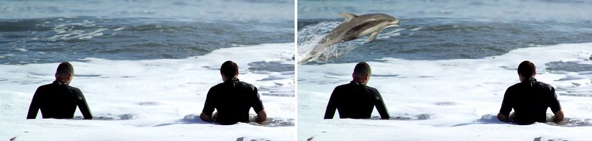
3

                            4                                                                       4
                                 (a)                                                                     (b)

                            3                                                                       3
       difference (× 104)

                                                                               difference (× 104)
                            2                                                                       2

                            1                                                                       1

                            0                                                                       0
                             0              10              20        30                             0              10              20        30
                                                 quantization                                                            quantization

Fig. 1. Shown in panel (a) is the sum of squared differences between coefficients quantized by an amount q1 = 17, followed by a second quantization
in the range q2 ∈ [1, 30] (horizontal axis) – this difference reaches a minimum at q2 = q1 = 17. Shown in panel (b) is the sum of squared differences
between coefficients quantized initially by an amount q0 = 23 followed by q1 = 17, followed by quantization in the range q2 ∈ [1, 30] (horizontal axis) –
this difference reaches a minimum at q2 = q1 = 17 and a local minimum at q2 = q0 = 23, revealing the original quantization.

                                 original                        35                                            40                        45

                                   50                            55                                            60                        65

                                   70                            75                                            80                        85

Fig. 2. Shown in the top left panel is the original image from which a central 200 × 200 region was extracted, saved at JPEG quality 65, and re-inserted
into the image whose original quality was 85. Shown in each subsequent panel is the difference between this image and a re-saved version compressed at
different JPEG qualities in the range [35, 85]. At the originally saved quality of 65, the central region has a lower difference than the remaining image.

Colour Image Database (UCID) [20]. These color images are                     was removed, saved at a specified JPEG quality of Q0 , re-
each of size 512 × 384 and span a wide range of indoor and                    inserted into the image, and then the entire image was saved
outdoor scenes, Fig. 3. A central portion from each image                     at the same or different JPEG quality of Q1 . The MatLab
4
TABLE I
accuracy degrades with smaller quality differences and smaller
JPEG GHOST DETECTION ACCURACY (%)
tampered regions. Shown in Fig. 4(a) are ROC curves for a
tampered region of size 150 × 150 and a quality difference
Q1 − Q0
size 0 5 10 15 20 25
of 15. Shown in Fig. 4(b) are ROC curves for a tampered
200 × 200 99.2 14.8 52.6 88.1 93.8 99.9 region of size 100×100 and a quality difference of 10. In each
150 × 150 99.2 14.1 48.5 83.9 91.9 99.8 panel, the solid curve corresponds to the accuracy of detecting
100 × 100 99.1 12.6 44.1 79.5 91.1 99.8 the tampered region, and the dashed curve corresponds to
50 × 50 99.3 5.4 27.9 58.8 77.8 97.7
the accuracy of correctly classifying an authentic image. The
vertical dotted lines denote false positive rates of 10%, 5%,
and 1%. As expected, there is a natural tradeoff between
function imwrite was used to save images in the JPEG the detection accuracy and the false positives which can be
format. This function allows for JPEG qualities to be specified controlled with the threshold on the K-S statistic.
in the range of 1 to 100. The size of the central region ranged In order to create a seamless match with the rest of the
from 50 × 50 to 200 × 200 pixels. The JPEG quality Q1 was image, it is likely that the manipulated region will be altered
selected randomly in the range 40 to 90, and the difference after it has been inserted. Any such post-processing may
between JPEG qualities Q0 and Q1 ranged from 0 to 25, where disrupt the detection of JPEG ghosts. To test the sensitivity to
Q0 ≤ Q1 (i.e., the quality of the central region is less than the such post-processing, the tampered region was either blurred,
rest of the image, yielding quantization levels for the central sharpened, or histogram equalized after being inserted into the
region that are larger than for the rest of the image). Note that image. For tampered regions of size 100 × 100, the detection
this manipulation is visually seamless, and does not disturb improved slightly (with the same false positive rate of 1%).
any JPEG blocking statistics.
The next few examples illustrate the efficacy of detecting
Note that is assumed here that the same JPEG quali-
JPEG ghosts in visually plausible forgeries. In each example,
ties/tables were used in the creation and testing of an image,
the forgery was created and saved using Adobe Photoshop CS3
and that there is no shift in the tampered region from its
which employs a 12-point JPEG quality scale. The MatLab
original JPEG block lattice. The impact of these assumptions
function imwrite was then used to re-compress each image
will be explored below, where it is shown that they are not
on a 100-point scale. In order to align the original JPEG block
critical to the efficacy of the detection of JPEG ghosts.
lattice with the re-saved lattice, the image was translated to
After saving an image at quality Q1 , it was re-saved at
each of 64 possible spatial locations (between 0 and 7 pixels
qualities Q2 ranging from 30 to 90 in increments of 1. The
in the horizontal and vertical directions). The shift that yielded
difference between the image saved at quality Q1 and each
the largest K-S statistic was then selected.
image saved at quality Q2 was computed as specified by
Equation (4), with b = 16. The K-S statistic, Equation (5), was Shown in Fig. 5 are an original and doctored image. The
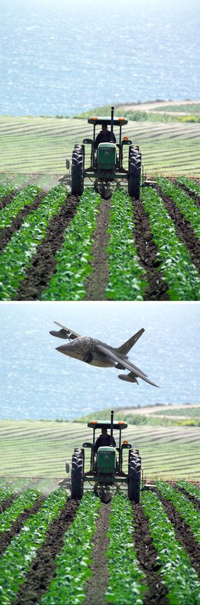
used to compute the statistical difference between the image’s inserted flying car was originally of JPEG quality 4/12 and
central region, and the rest of the image. If the K-S statistic the final image was saved at quality 10/12. Shown in the
for any quality Q2 exceeded a specified threshold, the image bottom portion of Fig. 5 are the difference images between the
was classified as manipulated. This threshold was selected to tampered image saved at JPEG qualities 60 through 98 in steps
yield a less than 1% false positive rate (an authentic image of 2. The maximal K-S statistic for the jet was 0.92. Regions
incorrectly classified as manipulated). of low variance are coded with mid-level gray in each panel.
Many of the images in the UCID database have significant A second example is shown in Fig. 6. The inserted dolphin
regions of either saturated pixels, or largely uniform intensity was originally of JPEG quality 5/12 and the final image was
patches. These regions are largely unaffected by varying JPEG saved at quality 8/12. Shown in the bottom portion of Fig. 6
compression qualities, and therefore exhibit little variation in are the difference images between the tampered image saved
the computed difference images, Equation (4). As such, these at JPEG qualities 60 through 100 in steps of 2. The maximal
regions provide unreliable statistics and were ignored when K-S statistic for the dolphin was 0.84. In both examples, the
computing the K-S statistic, Equation (5). Specifically, regions JPEG ghosts of the inserted car and dolphin are visually salient
of size b × b with an average intensity variance less than 2.5 and statistically distinct from the rest of the image.
gray values were simply not included in the computation of Shown in Fig. 7 are an original and doctored image. The jet
the K-S statistic. was originally of JPEG quality 6/12 and the final image was
Shown in Table I are the estimation results as a function of saved at quality 10/12. Shown in the middle portion of Fig. 7
the size of the manipulated region (ranging from 200 × 200 are the difference images between the tampered image saved at
to 50 × 50) and the difference in JPEG qualities between JPEG qualities 65 through 100 in steps of 5. The maximal K-S
the originally saved central region, Q0 , and the final saved statistic for the jet was 0.94. These panels correspond to the
quality, Q1 (ranging from 0 to 25 – a value of Q1 − Q0 = 0 correct spatial offset that aligns the original JPEG lattice with
denotes no tampering). Note that accuracy for images with no the re-saved lattices. Shown in the right-most portion of this
tampering (first column) is greater than 99% (i.e., a less than figure are the same difference images with incorrect spatial
1% false positive rate). Also note that the detection accuracy alignment. Notice that while the jet’s JPEG ghost is visible
is above 90% for quality differences larger than 20 and for when the alignment is correct, it largely vanishes when the
tampered regions larger than 100 × 100 pixels. The detection alignment is incorrect.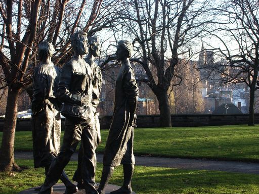
5
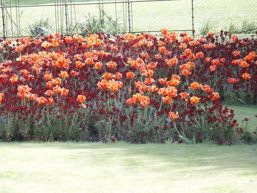
Fig. 3. Shown are representative examples from the 1, 000 UCID images.
(a) (b)
100 100
75 75
accuracy (%)
accuracy (%)
50 50
25 25
0 0
0 0.2 0.4 0.6 0 0.2 0.4 0.6 0.8
K!S statistic K!S statistic
Fig. 4. Shown are ROC curves for (a): a tampered region of size 150 × 150 and a quality difference of 15; and (b) a tampered region of size 100 × 100 and
a quality difference of 10. The solid curve corresponds to the accuracy of detecting the tampered region, and the dashed curve corresponds to the accuracy
of correctly classifying an authentic image. The vertical dotted lines denote (from left to right) false positive rates of 10%, 5%, and 1%. See also Table I.
IV. D ISCUSSION into which it was inserted. The advantage of this approach
is that it is effective on low quality images and can detect
We have described a simple and yet potentially powerful relatively small regions that have been altered. Because the
technique for detecting tampering in low quality JPEG images. JPEG ghosts are visually highly salient, an automatic detection
This approach explicitly detects if part of an image was algorithm was not implemented. It is likely that any of a
compressed at a lower quality than the saved JPEG quality variety of segmentation algorithms could be employed to
of the entire image. Such a region is detected by simply automatically detect JPEG ghosts and therefore automatically
re-saving the image at a multitude of JPEG qualities and and efficiently analyze a large number of images.
detecting spatially localized local minima in the difference
between the image and its JPEG compressed counterpart.
Under many situations, these minima, termed JPEG ghosts, ACKNOWLEDGMENT
are highly salient and easily detected. This work was supported by a gift from Adobe Systems,
The disadvantage of this approach is that it is only effective Inc., a gift from Microsoft, Inc., a grant from the National
when the tampered region is of lower quality than the image Science Foundation (CNS-0708209), a grant from the U.S. Air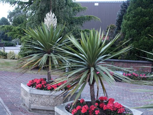
6

Force (FA8750-06-C-0011), and by the Institute for Security
Technology Studies at Dartmouth College under grants from
the Bureau of Justice Assistance (2005-DD-BX-1091) and
the U.S. Department of Homeland Security (2006-CS-001-
000001). Points of view or opinions in this document are those
of the author and do not represent the official position or poli-
cies of the U.S. Department of Justice, the U.S. Department
of Homeland Security, or any other sponsor.

                              R EFERENCES
 [1] J. Fridrich, D. Soukal, and J. Lukás̆, “Detection of copy-move forgery in
     digital images,” in Proceedings of Digital Forensic Research Workshop,
     August 2003.
 [2] A. C. Popescu and H. Farid, “Exposing digital forgeries by detecting
     duplicated image regions,” Department of Computer Science, Dartmouth
     College, Tech. Rep. TR2004-515, 2004.
 [3] T.-T. Ng and S.-F. Chang, “A model for image splicing,” in IEEE
     International Conference on Image Processing, Singapore, October
     2004.
 [4] İ. Avcıbaş, S. Bayram, N. Memon, B. Sankur, and M. Ramkumar, “A
     classifier design for detecting image manipulations,” in 2004 Interna-
     tional Conference on Image Processing, vol. 4, 2004, pp. 2645–2648.
 [5] A. C. Popescu and H. Farid, “Exposing digital forgeries by detecting
     traces of re-sampling,” IEEE Transactions on Signal Processing, vol. 53,
     no. 2, pp. 758–767, 2005.
 [6] ——, “Exposing digital forgeries in color filter array interpolated
     images,” IEEE Transactions on Signal Processing, vol. 53, no. 10, pp.
     3948–3959, 2005.
 [7] J. Lukáš, J. Fridrich, and M. Goljan, “Detecting digital image forgeries
     using sensor pattern noise,” in Proceedings of the SPIE, vol. 6072, 2006.
 [8] M. Johnson and H. Farid, “Exposing digital forgeries through chro-
     matic aberration,” in ACM Multimedia and Security Workshop, Geneva,
     Switzerland, 2006.
 [9] M. K. Johnson and H. Farid, “Exposing digital forgeries by detecting
     inconsistencies in lighting,” in ACM Multimedia and Security Workshop,
     2005.
[10] ——, “Exposing digital forgeries through specular highlights on the
     eye,” in 9th International Workshop on Information Hiding, Saint Malo,
     France, 2007.
[11] ——, “Exposing digital forgeries in complex lighting environments,”
     IEEE Transactions on Information Forensics and Security, vol. 2, no. 3,
     pp. 450–461, 2007.
[12] S. Ye, Q. Sun, and E. Chang, “Detecting digital image forgeries by mea-
     suring inconsistencies of blocking artifact,” in 2007 IEEE International
     Conference on Multimedia and Expo, 2007, pp. 12–15.
[13] W. Luo, Z. Qu, J. Huang, and G. Qiu, “A novel method for detect-
     ing cropped and recompressed image block,” in IEEE Conference on
     Acoustics, Speech and Signal Processing, 2007, pp. 217–220.
[14] J. He, Z. Lin, L. Wang, and X. Tang, “Detecting doctored JPEG images
     via DCT coefficient analysis,” in European Conference on Computer
     Vision, Graz, Austria, 2006.
[15] A. Popescu and H. Farid, “Statistical tools for digital forensics,” in 6th
     International Workshop on Information Hiding, Toronto, Cananda, 2004.
[16] “Digital compression and coding of continuous-tone still images, Part
     1: Requirements and guidelines,” ISO/IEC JTC1 Draft International
     Standard 10918-1, 1991.
[17] G. Wallace, “The JPEG still picture compression standard,” IEEE
     Transactions on Consumer Electronics, vol. 34, no. 4, pp. 30–44, 1991.
[18] W. Conover, Practical Nonparametric Statistics. John Wiley & Sons,
     1980.
[19] H. Farid, “Digital image ballistics from JPEG quantization,” Department
     of Computer Science, Dartmouth College, Tech. Rep. TR2006-583,
     2006.
[20] G. Schaefer and M. Stich, “UCID - an uncompressed colour image
     database,” School of Computing and Mathematics, Nottingham Trent
     University, U.K., Tech. Rep., 2003.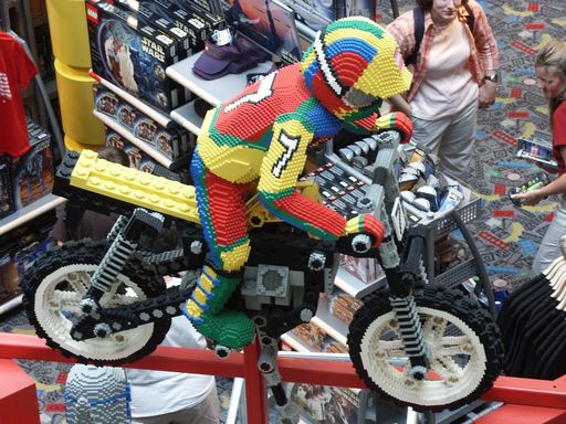
7

Fig. 5.   Shown are the original (left) and doctored (right) image. Shown below are the difference images at qualities 60 through 98 in steps of 2.
8

Fig. 6.   Shown are the original (left) and doctored (right) image. Shown below are the difference images at qualities 60 through 100 in steps of 2.
9

Fig. 7. Shown are the original (top left) and doctored (bottom left) image. Shown in the middle panels are the difference images at qualities 65 through
100 in steps of 5, and shown in the right-most panels are the difference images when the JPEG block lattice is mis-aligned.
You can also read