Daily report 11-04-2020 - Analysis and prediction of COVID-19 for different regions and countries

Daily report 11-04-2020
 Analysis and prediction of COVID-19 for
 different regions and countries

Situation report 26 Contact: clara.prats@upc.edu

 With the financial support of

Foreword
The present report aims to provide a comprehensive picture of the pandemic situation of COVID‐19 in the
EU countries, and to be able to foresee the situation in the next coming days.

We employ an empirical model, verified with the evolution of the number of confirmed cases in previous
countries where the epidemic is close to conclude, including all provinces of China. The model does not
pretend to interpret the causes of the evolution of the cases but to permit the evaluation of the quality of
control measures made in each state and a short-term prediction of tendencies. Note, however, that the
effects of the measures’ control that start on a given day are not observed until approximately 5-7 days later.

The model and predictions are based on two parameters that are daily fitted to available data:
  a: the velocity at which spreading specific rate slows down; the higher the value, the better the
 control.
  K: the final number of expected cumulated cases, which cannot be evaluated at the initial stages
 because growth is still exponential.

Next, we show a report with 8 graphs and a table with the short-term predictions for (1) European Union and
its countries, (2) other countries, (3) Spain and its autonomous communities.

We are currently adjusting the model to countries and regions with at least 4 days with more than 100
confirmed cases and a current load over 200 cases. The predicted period of a country depends on the number
of datapoints over this 100 cases threshold:
  Group A: countries that have reported more than 100 cumulated cases for 10 consecutive days or
 more → 3-5 days prediction;
  Group B: countries that have reported more than 100 cumulated cases for 7 to 9 consecutive days
 → 2 days prediction;
  Group C: countries that have reported more than 100 cumulated cases for 4 to 6 days → 1 day
 prediction.

We have introduced a change in fittings, that are now weighted at some points. The whole methodology
employed in the inform is explained in the last pages of this document.

Martí Català, MD Clara Prats, PhD
Pere-Joan Cardona, PhD Sergio Alonso, PhD
Comparative Medicine and Bioimage Centre of Enric Álvarez, PhD
Catalonia; Institute for Health Science Research Daniel López, PhD
Germans Trias i Pujol Computational Biology and Complex Systems;
 Universitat Politècnica de Catalunya - BarcelonaTech

With the collaboration of: Guillem Álvarez, Oriol Bertomeu, Laura Dot, Lavínia Hriscu, Helena Kirchner, Miquel
Marchena, Daniel Molinuevo, Pablo Palacios, Sergi Pradas, David Rovira, Xavier Simó, Tomás Urdiales

 PJC and MC received funding from “la Caixa” Foundation (ID 100010434), under agreement
 LCF/PR/GN17/50300003; CP, DL, SA, MC, received funding from Ministerio de Ciencia,
 Innovación y Universidades and FEDER, with the project PGC2018-095456-B-I00;

 1

(0) Executive summary – Dashboard

 2

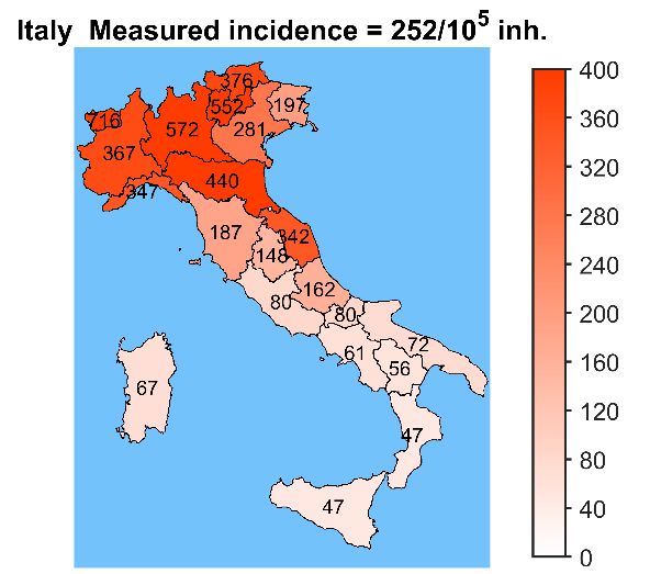
Global EU+EFTA+UK trends and needs
EU+EFTA+UK countries have reached a
global incidence of 142 cases per
100,000 inhabitants. As a response to
the fluctuations in new cases,
spreading rate is again at the
threshold between growth and
control (ρ≈1). This indicates a fragile
equilibrium between both states;
although global situation has
improved when compared with a few
weeks ago, it has not consolidated its
trend to control. This means that strict
watchfulness must be maintained,
especially in a moment where some
governments are studying or have
decided a relaxation of confinement
measures. In these countries, it is essential to maintain the control at a lower level, since regions can
individually be at different moments of the epidemiological cycle. In particular, despite a whole country may
have overtaken the peak, there can be regions with a ρ>1. This is the case, for instance, of some Italian and
Spanish regions (see report). Therefore, the relaxation of a control measure at the country level can prevent
those regions to enter the ρ

Situation and trends per country
Table of current situation in EU countries, according to data published by ECDC on April 11th. Colour scale is
relative except when indicated, this means that it is applied independently to each column, and distinguishes
best (green) form worst (red) situations according to each of the variables.
 Reported data Indexes
 Active cases Active cases
 Cumulated Attack rate / Cumulated Mortality
 Country 5 5 (last 10 (last 10 days) Mean ρ(1) EPG
 (2) (2)
 EPG2
 cases 10 inh. deaths /10 inh.
 days) /105 inh.
 Spain 157,022 338.8 15,843 34.2 62,605 135.1 0.75 101.7 76.6
 Italy 147,577 248.3 18,851 31.7 41,785 70.3 0.80 56.5 45.3
 Germany 117,658 143.6 2,544 3.1 50,292 61.4 0.80 49.1 39.3
 France 90,676 140.1 13,197 20.4 38,548 59.6 1.03 61.1 62.6
 United Kingdom 70,272 105.8 8,958 13.5 45,122 67.9 1.05 71.2 74.6
 Belgium 26,667 234.8 3,019 26.6 13,892 122.3 0.96 117.9 113.7
 Switzerland 24,228 282.7 805 9.4 8,120 94.7 0.63 59.5 37.4
 Netherlands 23,097 136.0 2,511 14.8 10,502 61.8 0.99 61.0 60.2
 Portugal 15,472 149.2 435 4.2 8,029 77.4 1.03 79.8 82.2
 Austria 13,560 155.6 319 3.7 3,378 38.8 0.90 35.1 31.7
 Sweden 9,685 98.4 870 8.8 5,250 53.4 1.24 66.2 82.1
 Ireland 8,089 171.2 287 6.1 4,854 102.7 1.57 161.3 253.4
 Norway 6,244 116.3 92 1.7 1,797 33.5 0.50 16.8 8.4
 Poland 5,955 15.6 181 0.5 3,644 9.5 1.02 9.8 10.0
 Denmark 5,819 101.9 247 4.3 2,959 51.8 0.97 50.0 48.3
 Czech Republic 5,732 54.0 119 1.1 2,424 22.8 0.88 20.2 17.8
 Romania 5,467 27.6 257 1.3 3,222 16.3 0.96 15.6 15.0
 Luxembourg 3,223 559.5 54 9.4 1,045 181.4 0.66 120.4 79.9
 Finland 2,769 50.3 48 0.9 1,385 25.2 1.51 38.0 57.5
 Greece 2,011 18.0 90 0.8 697 6.2 0.66 4.1 2.7
 Iceland 1,675 459.8 7 1.9 540 148.2 0.51 76.0 38.9
 Croatia 1,495 35.5 21 0.5 628 14.9 1.05 15.6 16.3
 Hungary 1,310 13.4 85 0.9 785 8.0 2.50 20.1 50.2
 Estonia 1,258 95.9 24 1.8 513 39.1 0.43 16.7 7.1
 Slovenia 1,160 55.8 45 2.2 346 16.7 0.86 14.4 12.4
 Lithuania 999 34.4 17 0.6 466 16.0 0.58 9.3 5.4
 Slovakia 715 13.1 2 0.0 352 6.5 2.30 14.8 34.1
 Bulgaria 635 8.9 25 0.4 236 3.3 0.81 2.7 2.2
 Latvia 612 31.1 2 0.1 214 10.9 0.69 7.5 5.1
 Cyprus 595 50.9 15 1.3 333 28.5 0.88 25.2 22.3
 Malta 350 81.6 2 0.5 183 42.7 ND ND ND
 Liechtenstein 80 207.5 1 2.6 12 31.1 ND ND ND

 Scale
 Worst Worst Worst Worst Worst Worst 2.0 200.0 200.0
 Best Best Best Best Best Best 0.0 0.0 0.0

(1)
 Disclaimer: parameter ρ is very sensitive and experiments daily variations. Mean ρ is averaged per 3 consecutive days,
but it can still vary the following days.
(2)
 EPG stands for Effective Growth Potential. It is obtained by multiplying attack rate per 105 inhabitants of last 10 days
(i.e. density of cases) by ρ (a value related with effective reproduction number and that, therefore, determines the
dynamics for subsequent days). EPG2 is a similar index but attack rate of last 10 days is multiplied by ρ2.

Highlights for countries with highest number of reported cases
  The 5 countries with more cases present predictions similar than yesterday, with UK at the level of
 4,800 (stable trend), Spain and Germany at the 4,600-4,000 (decreasing trend), France at the 3,800
 (stable trend) and Italy at the 3,600 (slow decreasing trend).
  Average ρ is still higher than 1 for both UK and France, while it is under 1 for Spain, Italy and Germany.

 4

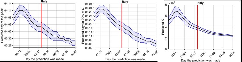
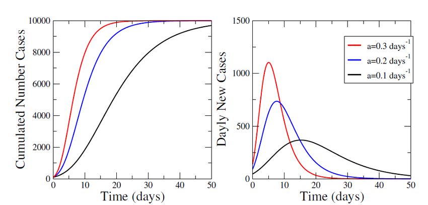
Analysis: Epidemiological dynamics analysis using Gompertz’s function. Reliability
of long-term predictions.
Gompertz’s function has proven to be a good tool for tracking the Covid-19 pandemic on a daily basis and
providing short-term predictions (up to 5 days) for the majority of affected countries. Its equation is as
follows:
 
 − � �· − ·( − 0)
 ( ) = 0

To make daily predictions we fit the function to the last 15 available data points assigning greater weight to
the last 3 ones in order to capture changes in trends quickly.

In this analysis we discuss the possibility of using Gompertz’s function to also make long-term predictions of:
(1) new cases’ peaks, (2) final incidence value and (3) approximate date when 90% of total final incidence will
be reached. In all three cases we are dealing with the evaluation of global dynamics, which requires small
changes in methodology: all data points be used instead of last 15 and with equal weight distribution among
them.

(1) New cases’ peak prediction, 

By computing the derivative of the function, we obtain the number of new cases over time. Its behaviour can
be observed in the following graphs (left, cumulated confirmed cases; right, its derivative):

We can calculate when the maximum new cases per unit of time will occur ( ) by using the second
derivative of the function:

 ln � � ��
 0
 = 0 +
 
(2) Final incidence value prediction, K

The parameter represents the total number of cases. Therefore, the fitting itself provides an estimation of
this value.

(3) 90% of total incidence date prediction

Gompertz’s function is asymptotical, it never reaches its maximum value. To estimate the duration of the
epidemic, a threshold value must be chosen. For example, we can calculate when 90% of total cumulated
cases will be reached ( 90 ). Solving algebraically, one obtains:

 6

− (0.9)
 � �
 ( / 0 )
 90 = 0 −
 
We have calculated these three different parameters for UE+EFTA+UK countries. In fact, we have gone back
in time to study how the estimation of each of them would evolve over time. Next is the evolution of said
predictions for Italy (left: ; centre, 90 ; right: ). The red line indicates the last estimate of in the
timeline (28th March).

These figures show that Italy has in fact already surpassed the predicted .

In this example we can observe how the estimated , 90 and decrease as the epidemic develops and
converge to a given value. Before overtaking the peak, the accuracy is substantially lower but after having
done so, the fitting improves with each new day. Therefore, we find that it is not possible to predict the peak
with reasonable accuracy until it has been passed. Thus, we cannot call it a prediction per se but a simple
proof that it has already passed. In fact, we have confirmed that the values of these parameters can only be
taken to be predictive of reality once the epidemic has reached the point of maximum new cases per day
(peak). Therefore, we can speak of a prediction of K and t90, but only once the peak has been overcome and
assuming that convergence towards a final value is progressive and improves as time passes.

At the end of this analysis we show similar figures for others countries.

The graphs in next page show predictions of , 90 and for the countries of the UE+EFTA+UK group
where it was possible to so 1 with the data available as of April 10th. The vertical line indicates the day in which
predictions are made and, therefore, shows which countries have surpassed the peak of the epidemic.
Furthermore, in these cases and 90 estimates would already be converging towards their final values.

1
 Predictions for countries that accomplish one of these criteria have been discarded: (a) current incidence is lower
than 25 % of K, (b) > 0.5 , (c) > 7 , (d) 90 > 7 .

 7

8

2020-04-10

 9

Situation and tendencies in Italian and Spanish regions
Italy. Data from 11/04/2020

 Reported data Indexes
 Active cases
 Attack rate Cumulated Mortality Active cases
 Country Cumulated cases 5 5
 (last ten days) Mean ρ(1) EPG(2) EPG2(2)
 / 10 inh. deaths / 10 inh. (last ten days)
 / 105 inh
 Lombardia 57,592 573.5 10,511 104.7 12,819 127.7 0.88 112.4 98.9
 Emilia Romagna 19,635 440.3 2,481 55.6 4,848 108.7 0.75 81.3 60.8
 Piemonte 16,008 367.5 1,633 37.5 6,213 142.6 0.90 129.0 116.7
 Veneto 13,768 280.6 831 16.9 4,143 84.5 1.22 103.4 126.5
 Toscana 6,958 186.6 467 12.5 2,091 56.1 0.93 52.4 49.0
 Liguria 5,376 346.7 734 47.3 1,716 110.7 0.77 85.7 66.3
 Marche 5,211 341.6 689 45.2 1,249 81.9 0.95 77.5 73.3
 Lazio 4,723 80.3 273 4.6 1,459 24.8 0.95 23.5 22.2
 Campania 3,517 60.6 238 4.1 1,286 22.2 0.57 12.7 7.3
 Trento 2,970 277.0 284 26.5 1,100 102.6 1.26 129.1 162.3
 Puglia 2,904 72.1 253 6.3 958 23.8 1.06 25.2 26.8
 Friuli Venezia Giulia 2,393 196.9 185 15.2 708 58.3 0.74 43.1 31.9
 Sicilia 2,364 47.3 154 3.1 646 12.9 0.99 12.8 12.7
 Abruzzo 2,120 161.6 206 15.7 684 52.2 1.26 65.9 83.2
 Bolzano 1,957 1,821.5 200 186.2 539 501.7 0.89 445.1 394.8
 Umbria 1,309 148.4 52 5.9 214 24.3 0.34 8.2 2.8
 Sardegna 1,091 66.5 73 4.5 346 21.1 1.04 22.1 23.0
 Calabria 915 47.0 66 3.4 246 12.6 0.70 8.9 6.3
 Valle d'Aosta 902 718.1 107 85.2 271 215.8 0.51 110.0 56.0
 Basilicata 312 55.4 17 3.0 75 13.3 0.57 7.6 4.3
 Molise 246 80.5 14 4.6 86 28.1 0.32 9.0 2.9

 Scale
 Worst Worst Worst Worst Worst Worst 2 700.0 900.0
 Best Best Best Best Best Best 0 0.0 0.0

Spain. Data from 11/04/2020

 Reported data Indexes
 Active cases
 Autonomous Total cumulated Attack rate Cumulated Mortality rate Active cases
 5 5
 (last 10 days) Mean ρ
 (1)
 EPG
 (2)
 EPG(2)
 regions cases /10 inh. deaths /10 inh. (last 10 days)
 /105 inh.
 Madrid 45,849 690.4 6,084 91.6 16,009 241.1 0.78 188.7 147.7
 Catalunya 32,984 436.0 3,331 44.0 12,993 171.7 0.90 155.1 140.1
 Castilla-La Mancha 13,456 661.1 1,483 72.9 6,409 314.9 0.83 259.9 214.6
 Castilla y Leon 11,543 479.3 1,180 49.0 4,696 195.0 1.08 210.1 226.3
 Euskadi 10,515 482.8 765 35.1 3,677 168.8 0.88 148.8 131.2
 Andalucia 9,712 115.3 737 8.7 3,320 39.4 0.5 21.2 11.4
 Comunitat Valenciana 8,578 172.4 818 16.4 2,656 53.4 0.99 52.6 51.9
 Galicia 7,176 265.7 261 9.7 2,744 101.6 0.58 59.3 34.6
 Aragon 3,969 300.5 425 32.2 1,478 111.9 0.74 82.5 60.8
 Navarra 3,817 587.3 227 34.9 1,320 203.1 0.87 177.1 154.4
 La Rioja 3,223 1,027.8 207 66.0 1,263 402.8 0.56 227.1 128.0
 Extremadura 2,486 233.3 303 28.4 807 75.7 1.15 86.8 99.5
 Canarias 1,887 85.5 95 4.3 507 23.0 0.85 19.4 16.5
 Asturias 1,827 178.7 128 12.5 505 49.4 0.5 25.9 13.5
 Cantabria 1,719 295.5 107 18.4 506 87.0 0.87 75.9 66.1
 Baleares 1,507 126.9 102 8.6 376 31.7 1.25 39.7 49.7
 Murcia 1,413 95.0 94 6.3 372 25.0 0.70 17.4 12.1
 Melilla 98 115.7 2 2.4 36 42.5 ND ND ND
 Ceuta 93 109.6 4 4.7 42 49.5 ND ND ND

 Scale
 Worst Worst Worst Worst Worst Worst 1.5 600.0 600.0
 Best Best Best Best Best Best 0.0 0.0 0.0

(1)
 Disclaimer: parameter ρ is very sensitive and experiments daily variations. Mean ρ is averaged per 3 consecutive days,
but it can still vary the following days. (2) EPG stands for Effective Growth Potential. It is obtained by multiplying attack
rate per 105 inhabitants of last 10 days (i.e. density of cases) by ρ (a value related with effective reproduction number
and that, therefore, determines the dynamics for subsequent days). EPG2 is a similar index but attack rate of last 10
days is multiplied by ρ2.

 10

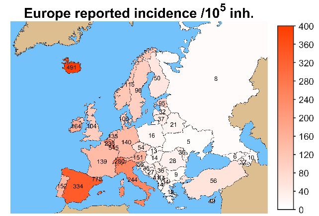
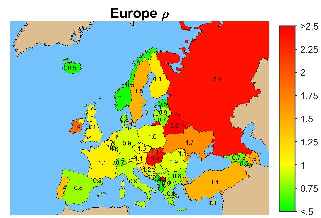
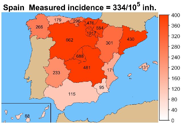
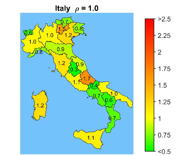
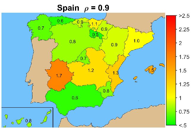
Maps of Italian and Spanish regions
Cumulated incidence and spreading rate (ρ) in Europe, Italian regions and Spanish autonomous communities.
Data from 10/04/2020.

 11

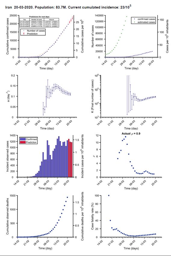
Legend: Countries’ reports details

Confirmed cases:
 data (blue), Estimated
 model fitted cases using
 (dashed line), death rate (see
predictions (red Methods)
points and table)

 Fitted a value Fitted K value
 using points using points
 prior to each prior to each
 date date

 Evolution of ρ, a
 Reported
 parameter related
 and
 with Reproduction
 predicted
 number (see
 new cases
 Methods)

 Reported Deaths /
 deaths cumulated
 reported cases

 12

(1) Analysis and prediction of COVID-19
 for EU+EFTA+UK

Data obtained from https://www.ecdc.europa.eu/en/geographical-distribution-2019-ncov-cases

 https://github.com/pcm-dpc/COVID-19/tree/master/dati-andamento-nazionale (Italy)

 13

14

15

16

17

18

19

20

21

22

23

24

25

26

27

28

29

30

31

32

33

34

35

36

37

38

39

40

41

42

43

44

45

(2) Analysis and prediction of COVID-19
 for other countries

Data obtained from https://www.ecdc.europa.eu/en/geographical-distribution-2019-ncov-cases

 46

47

48

49

50

51

52

53

54

55

56

57

58

59

60

61

62

(3) Analysis and prediction of COVID-19
 for Spain and its autonomous
 communities

Data obtained from https://github.com/datadista/datasets/tree/master/COVID%2019 and
 https://www.mscbs.gob.es/profesionales/saludPublica/ccayes/alertasActual/nCov-
 China/situacionActual.htm

 63

64

65

66

67

68

69

70

71

72

73

74

75

76

77

78

79

80

81

Methods

 82

Methods
(1) Data source
Data are daily obtained from World Health Organization (WHO) surveillance reports 2, from European Centre
for Disease Prevention and Control (ECDC) 3 and from Ministerio de Sanidad 4. These reports are converted
into text files that can be processed for subsequent analysis. Daily data comprise, among others: total
confirmed cases, total confirmed new cases, total deaths, total new deaths. It must be considered that the
report is always providing data from previous day. In the document we use the date at which the datapoint
is assumed to belong, i.e., report from 15/03/2020 is giving data from 14/03/2020, the latter being used in
the subsequent analysis.

(2) Data processing and plotting
Data are initially processed with Matlab in order to update timeseries, i.e., last datapoints are added to
historical sequences. These timeseries are plotted for EU individual countries and for the UE as a whole:

  Number of cumulated confirmed cases, in blue dots
  Number of reported new cases
  Number of cumulated deaths

Then, two indicators are calculated and plotted, too:

  Number of cumulated deaths divided by the number of cumulated confirmed cases, and reported as
 a percentage; it is an indirect indicator of the diagnostic level.
  ρ: this variable is related with the reproduction number, i.e., with the number of new infections
 caused by a single case. It is evaluated as follows for the day before last report (t-1):
 ( ) + ( − 1) + ( − 2)
 ( − 1) =
 ( − 5) + ( − 6) + ( − 7)
 where Nnew(t) is the number of new confirmed cases at day t.

(3) Classification of countries according to their status in the epidemic cycle
The evolution of confirmed cases shows a biphasic behaviour:

 (I) an initial period where most of the cases are imported;
 (II) a subsequent period where most of new cases occur because of local transmission.

Once in the stage II, mathematical models can be used to track evolutions and predict tendencies. Focusing
on countries that are on stage II, we classify them in three groups:

 • Group A: countries that have reported more than 100 cumulated cases for 10 consecutive days or
 more;
 • Group B: countries that have reported more than 100 cumulated cases for 7 to 9 consecutive days;
 • Group C: countries that have reported more than 100 cumulated cases for 4 to 6 days.

2
 https://www.who.int/emergencies/diseases/novel-coronavirus-2019/situation-reports
3
 https://www.ecdc.europa.eu/en/geographical-distribution-2019-ncov-cases
4
 https://www.mscbs.gob.es/profesionales/saludPublica/ccayes/alertasActual/nCov-China/situacionActual.htm
https://github.com/datadista/datasets/tree/master/COVID%2019

 83

(4) Fitting a mathematical model to data

Previous studies have shown that Gompertz model 5 correctly describes the Covid-19 epidemic in all analysed
countries. It is an empirical model that starts with an exponential growth but that gradually decreases its
specific growth rate. Therefore, it is adequate for describing an epidemic that is characterized by an initial
exponential growth but a progressive decrease in spreading velocity provided that appropriate control
measures are applied.

Gompertz model is described by the equation:
 
 − � �· − ·( − 0)
 ( ) = 0

where N(t) is the cumulated number of confirmed cases at t (in days), and N0 is the number of cumulated
cases the day at day t0. The model has two parameters:

  a is the velocity at which specific spreading rate is slowing down;
  K is the expected final number of cumulated cases at the end of the epidemic.

This model is fitted to reported cumulated cases of the UE and of countries in stage II that accomplish two
criteria: 4 or more consecutive days with more than 100 cumulated cases, and at least one datapoint over
200 cases. Day t0 is chosen as that one at which N(t) overpasses 100 cases. If more than 15 datapoints that
accomplish the stated criteria are available, only the last 15 points are used. The fitting is done using Matlab’s
Curve Fitting package with Nonlinear Least Squares method, which also provides confidence intervals of
fitted parameters (a and K) and the R2 of the fitting. At the initial stages the dynamics is exponential and K
cannot be correctly evaluated. In fact, at this stage the most relevant parameter is a. Fitted curves are
incorporated to plots of cumulative reported cases with a dashed line. Once a new fitting is done, two plots
are added to the country report:

  Evolution of fitted a with its error bars, i.e., values obtained on the fitting each day that the analysis
 has been carried out;
  Evolution of fitted K with its error bars, i.e., values obtained on the fitting each day that the analysis
 has been carried out; if lower error bar indicates a value that is lower than current number of cases,
 the error bar is truncated.

These plots illustrate the increase in fittings’ confidence, as fitted values progressively stabilize around a
certain value and error bars get smaller when the number of datapoints increases. In fact, in the case of
countries, they are discarded and set as “Not enough data” if a>0.2 day-1, if K>106 or if the error in K
overpasses 106.

It is worth to mention that the simplicity of this model and the lack of previous assumptions about the Covid-
19 behaviour make it appropriate for universal use, i.e., it can be fitted to any country independently of its
socioeconomic context and control strategy. Then, the model is capable of quantifying the observed
dynamics in an objective and standard manner and predicting short-term tendencies.

(5) Using the model for predicting short-term tendencies
The model is finally used for a short-term prediction of the evolution of the cumulated number of cases. The
predictions increase their reliability with the number of datapoints used in the fitting. Therefore, we consider
three levels of prediction, depending on the country:

5
 Madden LV. Quantification of disease progression. Protection Ecology 1980; 2: 159-176.

 84

• Group A: prediction of expected cumulated cases for the following 3-5 days 6;
 • Group B: prediction of expected cumulated cases for the following 2 days;
 • Group C: prediction of expected cumulated cases for the following day.

The confidence interval of predictions is assessed with the Matlab function predint, with a 99% confidence
level. These predictions are shown in the plots as red dots with corresponding error bars, and also gathered
in the attached table. For series longer than 9 timepoints, last 3 points are weighted in the fitting so that
changes in tendencies are well captured by the model.

(6) Estimating non-diagnosed cases
Lethality of Covid-19 has been estimated at around 1 % for Republic of Korea and the Diamond Princess
cruise. Besides, median duration of viral shedding after Covid-19 onset has been estimated at 18.5 days for
non-survivors 7 in a retrospective study in Wuhan. These data allow for an estimation of total number of
cases, considering that the number of deaths at certain moment should be about 1 % of total cases 18.5 days
before. This is valid for estimating cases of countries at stage II, since in stage I the deaths would be mostly
due to the incidence at the country from which they were imported. We establish a threshold of 50 reported
cases before starting this estimation.

Reported deaths are passed through a moving average filter of 5 points in order to smooth tendencies. Then,
the corresponding number of cases is found assuming the 1 % lethality. Finally, these cases are distributed
between 18 and 19 days before each one.

6
 At this moment we are testing predictions at 4 days for countries with more than 100 cumulated cases for 13-15
consecutive days, and 5 days for 16 or more days.
7
 Zhou et al., 2020. Clinical course and risk factors for mortality of adult
inpatients with COVID-19 in Wuhan, China: a retrospective
cohort study. The Lancet; March 9, doi: 10.1016/S0140-6736(20)30566-3

 85