A NEW METAHEURISTIC APPROACH FOR THE ART GALLERY PROBLEM
←
→
Page content transcription
If your browser does not render page correctly, please read the page content below
A N EW M ETAHEURISTIC A PPROACH FOR THE A RT G ALLERY
                                                               P ROBLEM

                                                                         B. Sadeghi Bigham∗, Sahar Badri, Nazanin Padkan
                                                                     Department of Computer Science and Information Technology
arXiv:2107.05540v2 [cs.CG] 19 Aug 2021

                                                                       Institute for Advanced Studies in Basic Sciences (IASBS)
                                                                                              Zanjan, Iran

                                                                                             August 20, 2021

                                                                                              A BSTRACT
                                                  In the problem "Localization and trilateration with the minimum number of landmarks", we faced
                                                  the 3-Guard and classic Art Gallery Problems. The goal of the art gallery problem is to find the
                                                  minimum number of guards within a simple polygon to observe and protect its entirety. It has many
                                                  applications in robotics, telecommunications, etc. There are some approaches to handle the art gallery
                                                  problem that is theoretically NP-hard. This paper offers an efficient method based on the Particle
                                                  Filter algorithm which solves the most fundamental state of the problem in a nearly optimal manner.
                                                  The experimental results on the random polygons generated by Bottino et al. [1] show that the new
                                                  method is more accurate with fewer or equal guards. Furthermore, we discuss resampling and particle
                                                  numbers to minimize the run time.
                                                  Keywords Art Gallery Problem · Localization · Visibility Polygon · Robotics · Particle Filter

                                         ∗
                                             Corresponding author,Email: b_sadeghi_b@iasbs.ac.ir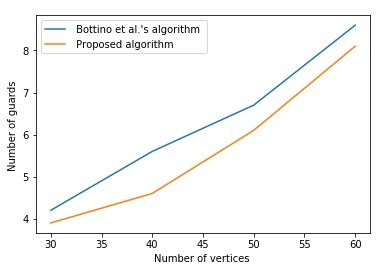
A PREPRINT - AUGUST 20, 2021

                                 Table 1: Symbols and variables used throughout the paper
              Symbols            Description
              P                  A simple polygon
              n                  The number of polygon vertices
              N                  The number of particles
              M                  The number of guards in the worst case
              |P |               Polygon’s area
              k                  The counter of guard numbers
              Xi                 A particle
              [xi , yi ]         A random point
              X                  A set of N particles
              V P (Xi )          Visibility polygon for particle Xi
              V P ([xi , yi ])   Visibility polygon for point [xi , yi ]
              wi                 Weight or importance of a particle
              vp(Xi )            The ratio of visibility area for particle Xi
              RN                 The resampling number
              vpmax              The best ratio for visibility area
              Best(X)            The best particle (with most coverage) in X
              τ                  Threshold or the acceptable percentage for entering the resampling stage

1   Introduction

The classical Art Gallery problem was posed by Victor Klee in 1973 [2] and has been studied for several decades as one
of the most important issues in computational geometry. It has many applications in minimizing landmarks, trilateration
[3], pose estimation [4], and robot localization [5]. There are many ways to protect an art gallery. An effective way is
using security cameras. Equipping an art gallery with many cameras will be expensive and difficult to maintain. On the
other hand, if the number of cameras is small, some parts of the gallery may not be monitored. The goal is to find the
minimum number of cameras (guards) to protect an art gallery. Every point in an art gallery should be visible to at least
one guard. The art gallery may be considered as an n−gon, designated P for short, that can be with or without holes.
The question is that how many guards are sufficient to cover P [2].
There are several types of art gallery problems. The two − guard [6] problem in a simple polygon P requires two
guards on the boundary of P from the starting vertex u to the ending vertex v. One of the guards goes around the
boundary clockwise and the other counterclockwise, such that they are able to see each other. The line segment
connecting the two guards are lies completely in P all the time [6].
The three − guard problem in a simple polygon P asks whether three guards can move from a vertex u to another
vertex v such that the first and third guards are separately on two boundary chains of P from u to v and the second
guard is always kept to be visible from two other guards inside P [7].
The location of the guards in the variations of the art gallery problem is different. Guards can be located on the vertices
of the polygon (vertex-guard), only on the edge (edge-guard), or without any restrictions (point-guard).
It has been known that the art gallery problem lies within the N P −hard problems. N P −hard problems are not
solvable in polynomial times. Lee and Lin [8] constructed a reduction from 3 − SAT and proved that the art gallery
problem is N P −hard. Finding the exact solution to these algorithms is time-consuming. Therefore, approximation and
metaheuristic algorithms are used to find approximate solutions to some hard optimization problems. These algorithms
can find near-optimal solutions in lower times. In 2018, Mikkel et al. [9] proved that the problem is ∃R−complete. The
class ∃R−complete consists of problems that can be reduced in polynomial times to the problem of deciding whether a
system of polynomial equations with integer coefficients and any number of real variables has a solution [9].
The art gallery problem has been widely studied over the years. In 1975, Chvátal established a theorem known as
Chvátal’s Art Gallery Problem [10]. It states that M = b n3 c guards are always sufficient and sometimes necessary
to protect an n−gon art gallery. In 1978, another simple proof based on the polygon triangulation and coloring of
vertices was proposed by Fisk [11]. Based on Fisk’s proof, Avis and Toussaint [12] proposed an O(n log n) time
divide-and-conquer algorithm for placing guards in a simple polygon.
The art gallery problem has also been studied for orthogonal polygons [13]. As an important subclass of polygons,
orthogonal polygons have internal angles of either 90◦ or 270◦ [14]. In 1983, Kahn et al. [15] proved that M = b n4 c
guards are always sufficient and sometimes necessary to protect an orthogonal polygon (galley). Later in 1983,

                                                            2
A PREPRINT - AUGUST 20, 2021
O’Rourke [13] proved again that the maximum guards in orthogonal polygons are M = b n4 c. Katz and Roisman [16]
proved that the art gallery problem for orthogonal polygons is N P −hard.
Gosh [17] proposed an approximation algorithm for the vertex-guard problem. Antonio et al. [18] presented an
approximation algorithm based on general metaheuristic genetic algorithms to solve the vertex-guard problem. Amit et
al. [19] introduced a heuristics algorithm for solving the point-guard problem. In 2011, Bottino et al. [1] introduced
optimal solutions for the point-guard problem and in 2013 Tozoni et al. [20] introduced an algorithm that successfully
found the exact solution when tested on a very large collection of instances from publicly available benchmarks, but
whose convergence could not be in general guaranteed.
The remaining sections of this paper are organized as follows: Some important definitions related to the article are
studied in Section 2. Then, in Section 3 a new metaheuristic method for the art gallery problem will be discussed and
the simulation results are studied in Section 4. The conclusion and future work are discussed in Section 5. All symbols
and variables used throughout the paper are introduced in Table 1.
2 Basic Definitions
In this section, some theoretical basics related to the proposed algorithm are going to be introduced.
2.1 Visibility Polygon
The visibility polygon is one of the foremost critical issues in computational geometry. Given a simple polygon P , two
points are said to be visible to each other if the line segment that joins them does not cross any obstacles [21]. Polygon
P will be covered by point q, if it is entirely visible from q. In 1980, the first algorithm for computing the visibility
polygon was introduced by Avis and ElGindy [22]. After that, different versions of this problem introduced each having
their own applications [23].
Consider P as an n−gon and q as a point in it. The goal is to compute the visibility polygon or the covered area. In
order to compute the visibility polygon in concave polygons, let P = (v0 , v1 , ..., vn ) and E = (v0 v1 , ..., vn−1 vn ) are
respectively as polygon’s vertices and edges. Asano et al. [24] introduced an algorithm (Algorithm 1) to compute the
visibility polygon in concave polygons using the Sweep Line algorithm which the complexity of it is O(n log n).
Algorithm 1 Computing the visibility polygon of a point q in a concave polygon P [24]
Input: Polygon P = (v0 , v1 , ..., vn ) and point q inside P
Output: Visibility Polygon V (P, q)
Sort (v0 , v1 , ..., vn ) counterclockwise
Save E in the queue
if P is convex then
V (P, q) = P
else
Draw lines from q to (v0 , v1 , ..., vn )
Save the lines in the new queue
if the lines are outside P then
Delete the lines
else
Save them in the new queue
end if
end if
Return V (P, q)
2.2 Particle Filter
The particle filter is a recursive algorithm that was introduced in 1996 by Del Moral [25] and has been widely used in
diverse fields such as robotics [26]. The general idea in this problem is to seek an approximate solution of a complex
model rather than an accurate solution of a simple model.
The particle filter uses a set of particles to find feasible solutions to a problem. Each particle provides a feasible solution
to the problem. Using the uniform random distribution, the algorithm spreads particles in the inner space of a polygon.
At first, the particles have the same weight. According to the information obtained, the particle weights are being
3A PREPRINT - AUGUST 20, 2021
changed and will be updated. So, the low-weighted particles are destroyed and are being produced again around the
high-weighted particles. This step is known as resampling.
In the following, using the theoretical foundations put forwarded, the proposed algorithm for the art gallery problem
will be introduced.
3 A New Algorithm for the Art Gallery Problem using the Particle Filter
First, some particles are uniformly distributed in the polygon space. The probability that each particle is a solution to
the problem is considered to be the same. For example, 50 particles are uniformly dispersed. So, the probability of each
1
particle being a solution is 50 that shows the particle weight or importance. Although each particle is regarded as a
feasible solution in the particle filter algorithm, each particle is considered as a set of points (guards) in the proposed
algorithm. Consider n−gon P as the input of the algorithm.
As mentioned before, M = b n3 c guards are needed to protect an n−gon in the worst case. The number of guards in
each stage is represented by k. The maximum value of k is M . The binary search is done in each stage until reaches an
optimal solution.
3.1 Binary Search
The binary search algorithm is used to find the optimal solution (optimal k) in an ordered array (this set is started from
1 to M ). In the binary search, the search space is split in half ( M M
2 ). First, 2 guards are checked that can cover the
polygon or not. If 2 guards are enough to cover the polygon, the first split ([1, 2, ..., M
M
2 ]) is divided into two minor sets
again and the binary search will be continued. If M 2 guards are not adequate, the second split ([ M
2 , ..., M ]) is divided
into two minor sets again and the binary search will be continued. This process is continued until the optimal number of
guards are obtained or all the elements are checked.
Let X be a set of N particles:
X = (X1 , X2 , ..., XN )
Then, the particles are monotonously distributed in the polygon and the particle weights are defined as follows:
1
wi = N st 1 ≤ i ≤ N
Each particle is regarded as a set of M random points (guards) in the polygon such as an M −footed spider as follows:
[1] [1] [1] [1] [1] [1]
X1 = ([x1 , y1 ], [x2 , y2 ], ..., [x[M ] , y[M ] ])
[2] [2] [2] [2] [2] [2]
X2 = ([x1 , y1 ], [x2 , y2 ], ..., [x[M ] , y[M ] ])
.
.
.
[N ] [N ] [N ] [N ] [N ] [N ]
XN = ([x1 , y1 ], [x2 , y2 ], ..., [x[M ] , y[M ] ]).
Using the the Algorithm 1, the visibility polygon of each particle is computed by the union of the visibility polygons of
the set of its points.
[1] [1] [1] [1] [1] [1]
V P (X1 ) = V P ([x1 , y1 ]) ∪ V P ([x2 , y2 ]) ∪ V P... ∪ V P ([x[M ] , y[M ] ])
[2] [2] [2] [2] [2] [2]
V P (X2 ) = V P ([x1 , y1 ]) ∪ V P ([x2 , y2 ]) ∪ V P... ∪ V P ([x[M ] , y[M ] ])
.
.
.
[N ] [N ] [N ] [N ] [N ] [N ]
V P (XN ) = V P ([x1 , y1 ]) ∪ V P ([x2 , y2 ]) ∪ V P... ∪ V P ([x[M ] , y[M ] ]).
Then, the particle weights are being updated:
vp(X1 ) = (|V P (X1 ))|P |
4A PREPRINT - AUGUST 20, 2021
vp(X2 ) = (|V P (X2 ))|P |
.
.
.
vp(XN ) = (|V P (XN ))|P |.
For each particle Xi , the weight vp(Xi ) is obtained from the ratio of the area of the visibility polygon for each particle
(|V P (Xi )|) to the area of the polygon |P |. Then, the resampling stage is started and repeated until vp(max) = 1
(the best ratio for the visibility area). The counter of the resampling stages is j. It is started from 1 and is updated by
incrementing by 1 at each stage until it reaches the maximum defined number RN (the defined resampling number).
The best particle X is obtained when vp(Xi ) = 1 which is indicative a feasible solution to the problem. No other
particles are needed to be checked. There is no need to complete the sampling at this stage.
If vp(max) 6= 1, then there will be two states:
• All the resampling stages RN are completed and the particle that covers the polygon is obtained and there is
no need to check the other particles.
• All the resampling stages RN are completed, but the particle that covers the polygon is not obtained yet.
Therefor, the particle that covered the polygon in the last stage is selected as the optimal solution (Best X).
Algorithm 2 Minimum Guards for the Art Gallery Problem
Input: Simple polygon P with n vertices
Output: Location of the minimum number of guards to guard P
kmin = 1, kmax = bn/3c and k = kmax+kmin 2
while 1 do
Generate X = {X1 , X2 , ..., XN }.
for j = 1; j = RN ; j + + do
vpmax (X) = 0
for i = 1; i = N ; i + + do
vp(Xi ) = |V P|P(X| i )|
if vp(Xi ) > vpmax (X) then
vpmax (X) = vp(Xi )
end if
if vpmax (X) == 1 then
BestX = Xi ;
break(); /* No need to other particles */
end if
end for
if vpmax (X) == 1 then
kmax = k;
kopt = k;
break(); /* No need to other resampling */
else
kmin = k;
end if
end for
end while
Return(kopt); /* When any particle cannot cover P with k cameras*/
Return(BestX) /* The best result for previous k */
3.1.1 The Resampling Stage
In this stage, low-weighted particles will be eliminated and reproduced again around the high-weighted particles. For
example, high-weighted particles which their vp(Xi ) are more than a specific threshold such as τ = 0.9 (the particles
that cover more than 90% of the polygon) are sampled and the particles that cover the polygon lower than 90% will
be omitted. Then, the omitted particles are reproduced around the high-weighted particles. Therefore, the number of
particles N is constant and their locations are changed.
5A PREPRINT - AUGUST 20, 2021
In the following, the visibility polygon for each particle is computed using the Algorithm 1 (the weights are updated).
Another resampling stage is done again (The maximum number of the resampling stages is limited, for example 20). A
particle may be found that vp = 1 (the particle can cover the polygon). Then, this particle will be saved as an optimal
solution. Regard that this particle is not unique. This procedure will be performed for all particles using the binary
search. It is possible to obtain no particle after completing all the resampling stages. In this situation, the particle
that covered the polygon in the last stage is regarded as the optimal solution. The proposed approach is presented in
Algorithm 2. This algorithm finds the minimum number of required guards to protect a polygon using the particle filter
algorithm.
If vp < 0.9 or vp > 0.9 for all the particles, any particles can enter the resampling stage. Reproducing omitted particles
around other particles is based on their weights. The omitted particles are reproduced more around a particle which has
higher vp.
The complexity of the particle filter algorithm is O(N logN ) for N particles and the visibility polygon for an n−gon
can be computed in O(n log n) times. In the worst case, the steps are repeated O(log M ) times using the binary search
method in which M = n3 . The algorithm runs RN times which is resampling numbers and it is at most O(n/3). So, the
whole complexity of the proposed algorithm is O(n3 log2 n).
4 The Experimental Results
The simulation results are presented here to evaluate the proposed algorithm.
Example 1: According to [19], a simple polygon with 18 vertices is considered. The polygon’s area (P ) is 92243.5m
and its coordinates are as follows:
P = ([558, 497], [513, 148], [477, 413], [439, 413], [403, 150], [384, 410],
[339, 409], [298, 152], [267, 409], [228, 409], [192, 151], [161, 412]
[124, 412], [80, 151], [74, 413], [52, 413], [25, 147], [11, 497]).
According to M = b 18 3 c = 6 and the binary search algorithm, the proposed procedure for [1, 2, 3, ..., 6] is as follows.
The algorithm is first performed on 3D particles. If a particle can be found that covers the polygon, the algorithm will
be performed on the first part of the array [1, 2, 3] using the binary search. Here, the particle is not found, so the second
part of the array [3, 4, 5, 6] is checked using the binary search. In fact, the algorithm is examined for 5D particles. If a
5D particle that covers the polygon is found, then the algorithm will be performed for 4D particles. Since the covering
5D particle is not found here, the algorithm will be checked for 6D particles. After implementing the algorithm on
particle dimension using the binary search, it is concluded that the algorithm for 6D particles (6 guards) reaches the
optimal solution. The guards’ locations for the 6D particle are shown in Figure 1. Their coordinates are shown in
Best(x) = ([83, 402], [22, 276], [227, 414], [514, 231], [320, 360], [404, 487]).
Figure 1: The simulation results of the proposed algorithm for the given polygon in [19] shows that 6 guards (small
black diamonds) are needed to be selected in this polygon.
Example 2: According to Amit et al. [19], another simple polygon with 21 vertices is considered. The polygons’ area
(P ) is 91201.5m and its coordinates are as follows:
P = ([475, 512], [146, 512], [284, 486], [146, 480], [147, 366], [118, 415]
[99, 288], [128, 295], [146, 336], [151, 226], [256, 226], [151, 191], [405, 190], [294, 226], [438, 223], [437, 316],
[475, 230], [472, 418], [437, 343], [428, 474], [314, 480]).
According to M = b 21 3 c = 7 and the binary search algorithm, for [1, 2, 3, ..., 7] the proposed procedure is as follows.
The algorithm is first performed on the 4D particles. The 4D particle that covers the polygon is found, so the first
part of the array [1, 2, 3, 4] is examined using the binary search. The algorithm tries to find a 2D particle to cover the
6A PREPRINT - AUGUST 20, 2021
polygon. After detecting this particle, the algorithm tries to find a 1D particle that covers the polygon. Here, the 2D
particle to cover the polygon that covers the polygon is not found. Then, the algorithm is checked to detect a 3D particle
to cover the polygon and this particle is not found either. After implementing the algorithm on particle dimension
using the binary search, it is concluded that the algorithm for 4D particles (4 guards) reaches the optimal solution. The
guards’ locations for the 4D particle are shown in Figure 2. Their coordinates are
Best(X) = ([116, 348], [208, 209], [435, 324], [292, 495]).
Figure 2: The simulation results of the proposed algorithm for the given polygon in [19] shows that 4 guards (small
black diamonds) are needed to be located in this polygon.
Figure 3: Comparison of the average guard numbers of the proposed algorithm with those in [1]
Using results obtained for the above examples and comparing them with Amit et al. [19], it can be inferred that the
results are approximately optimal.
A comparison between the average accuracy of the proposed algorithm and that of Bottino et al. [1] for random
polygons is shown in Table 2. In this comparison, 20 random 30−gons, 40−gons, 50−gons, and 60−gons are studied.
These polygons are the same as the ones in [1] and some of them are shown in Figure 4.
Table 2 shows that the average optimal number of guards for random polygons in the proposed algorithm is less than or
equal to the average optimal number of guards in [1] shown graphically in Figure 3.
Table 2: Comparison of the results of the method and Bottino et al. [1]
n Proposed method Bottino et al.’s algorithm [1]
30 3.9 4.2
40 4.6 5.6
50 6.1 6.7
60 8.1 8.6
7A PREPRINT - AUGUST 20, 2021
Figure 4: Some of the studied polygons and the locations of the guards using the proposed method.
Figure 5: According to the simulation results of the proposed algorithm, 6 guards are needed to be selected in this
50−gon.
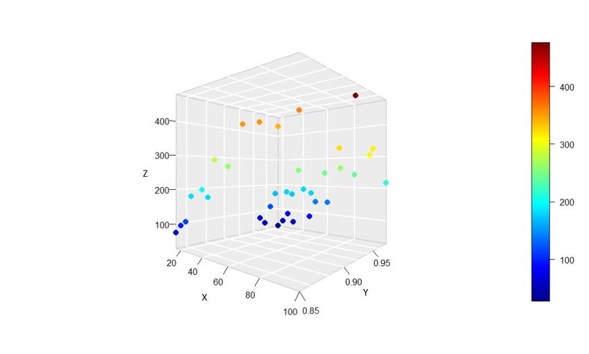
In the following, the proposed algorithm is examined on an arbitrary 50−gon (Figure 5) and apply it to the different
numbers of particles and thresholds (τ ). The optimal solutions are obtained at different times and illustrated in Figure 6.
As shown there, the X,Y, and Z axes indicate the number of particles, threshold (τ ), and time, respectively. The color
spectrum on the right shows the time in seconds and its color changes from blue to red with the increasing time. The
points in the range of 1 to 100 seconds are blue. As the time increases, the color changes from dark blue to light blue.
The darkest red point shows the optimal solution at the latest time (476 s) that is obtained when the number of particles
is 90 and τ = 0.95. The darkest blue point indicates the optimal solution with the minimum running time (28 s) and is
obtained when the number of particles is 15 and the threshold is set at τ = 0.98. Also, the darkest red point shows the
8A PREPRINT - AUGUST 20, 2021
worst solution and the longest time used (476 s) and is obtained when the number of particles is 90 and the τ is 0.95.
The results show that [N = n/3] and τ = 0.98% are acceptable settings for our algorithm. The achievements of this
paper can be used in issues such as SLAM and pose estimation.
Figure 6: The optimal solutions at different times
9A PREPRINT - AUGUST 20, 2021
5 Conclusion and Future Work
The art gallery problem is one of the most vital NP-hard problems in computational geometry applicable in robot
localization and SLAM. Using the particle filter, a new heuristic method has been proposed in this paper to find the near
optimal solution of the art gallery problem. In this method, each particle provides an optimal solution to find the number
and location of the adequate guards that would guard the given polygon. The experimental results show that our method
finds fewer (or equal) number of guards to achieve this goal. In future work, guarded guard problem, 2−Guards and
3−Guards problems may be considered. Also, one can extend our results to solve the problem of achieving maximum
coverage for a given polygon using a fixed number of guards.
6 Acknowledgements
The authors would like to express their sincerely gratitude to Dr. A. Bottino for providing the data that helped us make
a better comparison.
References
[1] Andrea Bottino and Aldo Laurentini. A nearly optimal algorithm for covering the interior of an art gallery. Pattern
recognition, 44:1048–1056, 2011.
[2] Joseph O’rourke. Art gallery theorems and algorithms, volume 57. Oxford University Press Oxford, 1987.
[3] B Sadeghi Bigham, S Dolatikalan, and A Khastan. Minimum landmarks for robot localization in orthogonal
environments. Evolutionary Intelligence, pages 1–4, 2021.
[4] Farhad Shamsfakhr and Bahram Sadeghi Bigham. Gsr: geometrical scan registration algorithm for robust and fast
robot pose estimation. Assembly Automation, 2020.
[5] Farhad Shamsfakhr, Bahram Sadeghi Bigham, and Amirreza Mohammadi. Indoor mobile robot localization in
dynamic and cluttered environments using artificial landmarks. Engineering Computations, 2019.
[6] Christian Icking and Rolf Klein. The two guards problem. International Journal of Computational Geometry &
Applications, 2:257–285, 1992.
[7] Xuehou Tan. An efficient algorithm for the three-guard problem. Discrete applied mathematics, 156:3312–3324,
2008.
[8] D Lee and Arthurk Lin. Computational complexity of art gallery problems. IEEE Transactions on Information
Theory, 32:276–282, 1986.
[9] Mikkel Abrahamsen, Anna Adamaszek, and Tillmann Miltzow. The art gallery problem is -complete. pages
65–73, 2018.
[10] Vasek Chvatal. A combinatorial theorem in plane geometry. Journal of Combinatorial Theory, Series B, 18:39–41,
1975.
[11] Steve Fisk. A short proof of chvátal’s watchman theorem. Journal of Combinatorial Theory, Series B, 24:374,
1978.
[12] David Avis and Godfried T Toussaint. An efficient algorithm for decomposing a polygon into star-shaped polygons.
Pattern Recognition, 13:395–398, 1981.
[13] Joseph O’Rourke. An alternate proof of the rectilinear art gallery theorem. Journal of Geometry, 21:118–130,
1983.
[14] T S Michael and Val Pinciu. The orthogonal art gallery theorem with constrained guards. Electronic Notes in
Discrete Mathematics, 54:27–32, 2016.
[15] Jeff Kahn, Maria Klawe, and Daniel Kleitman. Traditional galleries require fewer watchmen. SIAM Journal on
Algebraic Discrete Methods, 4:194–206, 1983.
[16] Matthew J Katz and Gabriel S Roisman. On guarding the vertices of rectilinear domains. Computational Geometry,
39:219–228, 2008.
[17] Subir Kumar Ghosh. Approximation algorithms for art gallery problems in polygons and terrains. International
Workshop on Algorithms and Computation, pages 21–34, 2010.
10A PREPRINT - AUGUST 20, 2021
[18] Antonio L Bajuelos, Santiago Canales, Gregorio Hernández, and Ana Mafalda Martins. Optimizing the minimum
vertex guard set on simple polygons via a genetic algorithm. WSEAS Transactions in Information Science and
Applications, 5:1584–1596, 2008.
[19] Yoav Amit, Joseph S B Mitchell, and Eli Packer. Locating guards for visibility coverage of polygons. International
Journal of Computational Geometry & Applications, 20:601–630, 2010.
[20] Davi C Tozoni, Pedro J de Rezende, and Cid C de Souza. The quest for optimal solutions for the art gallery
problem: A practical iterative algorithm. pages 320–336, 2013.
[21] Joseph O’Rourke. Visibility, 2017.
[22] Hossam El Gindy and David Avis. A linear algorithm for computing the visibility polygon from a point. Journal
of Algorithms, 2:186–197, 1981.
[23] Marzieh Eskandari and Mahdieh Yeganeh. S-visibility problem in vlsi chip design. Turkish Journal of Electrical
Engineering & Computer Sciences, 25:3960–3969, 2017.
[24] Tetsuo Asano. An efficient algorithm for finding the visibility polygon for a polygonal region with holes. IEICE
TRANSACTIONS (1976-1990), 68:557–559, 1985.
[25] Pierre Del Moral. Nonlinear filtering: Interacting particle resolution. Comptes Rendus de l’Académie des
Sciences-Series I-Mathematics, 325:653–658, 1997.
[26] Claudiu Pozna, Radu-Emil Precup, and Péter Földesi. A novel pose estimation algorithm for robotic navigation.
Robotics and Autonomous Systems, 63:10–21, 2015.
11You can also read