Extension of Sinkhorn Method: Optimal Movement Estimation of Agents Moving at Constant Velocity
←
→
Page content transcription
If your browser does not render page correctly, please read the page content below
Extension of Sinkhorn Method: Optimal
                                                 Movement Estimation of Agents Moving at
arXiv:1907.05036v1 [eess.IV] 11 Jul 2019

                                                             Constant Velocity

                                               Daigo Okada ∗1 , Naotoshi Nakamura †1 , Takuya Wada ‡2 , Ayako
                                                               Iwasaki §2 , and Ryo Yamada ¶1
                                                   1 Graduate
                                                           School of Medicine, Kyoto University, Syogoin
                                                Kawaharachoh 53, Sakyo, Kyoto, Kyoto Prefecture, Japan
                                           2 Department of Medicine, Kyoto University, Syogoin Kawaharachoh

                                                        53, Sakyo, Kyoto, Kyoto Prefecture, Japan

                                                                                  July 12, 2019

                                                                                      Abstract
                                                      In the field of bioimaging, an important part of analyzing the motion of objects
                                                 is tracking. We propose a method that applies the Sinkhorn distance for solving
                                                 the optimal transport problem to track objects. The advantage of this method is
                                                 that it can flexibly incorporate various assumptions in tracking as a cost matrix.
                                                 First, we extend the Sinkhorn distance from two dimensions to three dimensions.
                                                 Using this three-dimensional distance, we compare the performance of two types
                                                 of tracking technique, namely tracking that associates objects that are close to
                                                 each other, which conventionally uses the nearest-neighbor method, and tracking
                                                 that assumes that the object is moving at constant velocity, using three types of
                                                 simulation data. The results suggest that when tracking objects moving at constant
                                                 velocity, our method is superior to conventional nearest-neighbor tracking as long
                                                 as the added noise is not excessively large. We show that the Sinkhorn method can
                                                 be applied effectively to object tracking. Our simulation data analysis suggests that
                                                 when objects are moving at constant velocity, our method, which sets acceleration
                                                 as a cost, outperforms the traditional nearest-neighbor method in terms of tracking
                                                 objects. To apply the proposed method to real bioimaging data, it is necessary to
                                                 set an appropriate cost indicator based on the movement features.

                                           ∗ dokada@genome.med.kyoto-u.ac.jp
                                           † nnakamura@genome.med.kyoto-u.ac.jp
                                           ‡
                                               peacefield.taku3@gmail.com
                                           § iwasaki.ayako.38n@st.kyoto-u.ac.jp
                                           ¶ Corresponding   Author: ryamada@genome.med.kyoto-u.ac.jp

                                                                                          1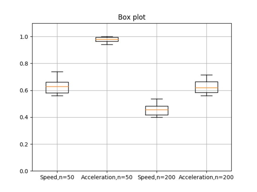
1 Introduction
In the field of bioimaging, an important part of analyzing the motion of objects is
tracking [1, 2, 3]. The tracking process can be described as follows. Images taken
at fixed time intervals contain many objects. The goal is to identify which signals
correspond to which object at the next time point. This task is important for bioimaging
analysis, such as the analysis of microscopy videos, because it is indispensable for
analyzing the motion of objects from image data taken at fixed time intervals. However,
automatic tracking is difficult. Many types of algorithm have been proposed for this
task [4, 5], including the nearest-neighbor method [6], probabilistic data association
[7], and multiple hypothesis tracking [8].
    Nearest-neighbor algorithms, the most simple of tracking methods, are used for
live-cell tracking in the field of bioimaging analysis [9]. These algorithms associate
objects that are close to each other. Although this is a simple task, the performance
of nearest-neighbor algorithms is inadequate when the objects are crowded together or
their movement distance is long. These difficult conditions are common in bioimaging
data. In this study, we extend the nearest-neighbor method. Because nearest-neighbor
tracking can be considered as an optimal transport algorithm, we adopt the Sinkhorn
method [10], an optimal transport algorithm, to modify nearest-neighbor tracking.
    In this research, we apply the Sinkhorn method to object tracking. This allows us
to perform tracking using various transport costs based on a model of object behavior.
For tracking, we do not have to associate the nearest objects at two consecutive time
points; we can associate objects so that their trajectories are smooth. A smooth trajec-
tory means that changes in velocity are small, or that the objects are moving at constant
velocity. Therefore, we use three consecutive time-point images to measure changes
in velocity, weigh the changes as a cost, and optimize the combination of spots in the
three time-point images using Sinkhorn regularization. In the following sections, we
describe the notation of the nearest-neighbor-based Sinkhorn approach and the exten-
sion of the Sinkhorn method to optimization for objects moving at constant velocity,
followed by methods for generating simulation datasets. We then compare the perfor-
mance of two Sinkhorn-based methods, namely the nearest-neighbor method and the
proposed method, using the datasets.

2 Theory/calculation
1. Overview of optimal transport problem and Sinkhorn method
Optimal transport has been investigated as a major problem in information science. It
can be applied to various fields [11], including tracking in imaging analysis [12]. The
optimal transport problem is as follows. Items are distributed in spots, which we call
sources. We want to move the items to new spots, which we call targets. What we
want to know is how many items should be moved from where to where. We want to
move the items with minimum cost. The cost is the sum of the products of the volume
of items and the distance between spots. The optimal transport problem can be defined
mathematically as follows. The source and target are discrete mass vectors r and c,

                                           2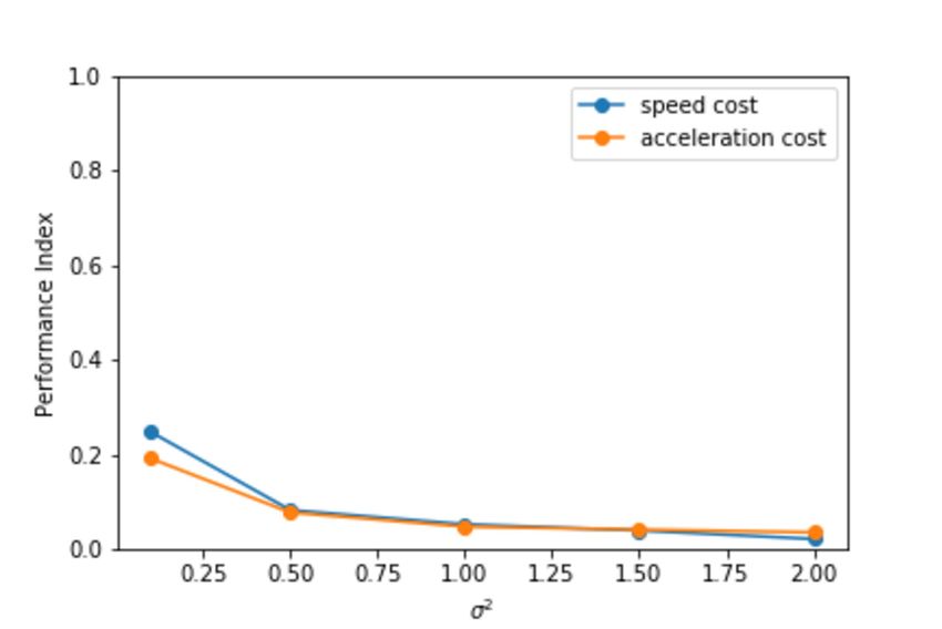
which satisfy the definition of a discrete probability distribution. Transportation, how
many items are moved from where to where, is expressed as matrix P, whose elements
represent the amount of movement from each source to each target. The elements
are non-negative and their row and column sums are the source and target vectors,
respectively. With the number of objects denoted as d, P is a d × d square matrix,
where the numbers of rows and columns of P correspond to the numbers of elements
of r and c, respectively. P is defined by the following equation:

                        U (r, c) := {P ∈ Rd×d ~        T~
                                          + |P1d = r, P 1d = c}                           (1)

 where Rd×d
          +    represents a set of matrices, whose elements are all non-negative, and
~1d represents a vector, whose elements are all 1. Each element of P represents the
 transportation of an object from one spot in r to one spot in c. Therefore, using cost
 matrix M, whose size is the same as that of P and whose elements represent the unit cost
 of the corresponding transportation, hP, Mi = ∑i, j pi j mi j is the Frobenius inner product
 of P and M where pi j and mi j are (i, j)th element of P and M, respectively, which
 represents the total cost. The optimal transportation matrix P∗ is defined as follows:

                   dM (r, c) = hP∗ , Mi,   where P∗ = arg minhP, Mi.                      (2)
                                                          P∈U(r,c)

The transport distance dM (r, c) [13] calculated using a cost matrix whose elements
are the distances of corresponding transportation of spots can be used as the distance
between r and c. Sinkhorn proposed an algorithm for the optimization of this distance
[10]. Because the search space of this optimization, U (r, c), is large, Sinkhorn added a
regularization term based on entropy and transformed the minimization of the transport
                                                         λ (r, c), as defined below. This
distance into the minimization of the Sinkhorn distance dM
regularization makes the area smaller and thus easier to search. The Sinkhorn distance
is defined as:

             λ                                                         1
            dM (r, c) = hPλ , Mi,    where Pλ = arg min(hP, Mi −         h (P)).          (3)
                                                    P∈U(r,c)           λ

where h (P) is the entropic term ∑di, j=1 pi j log pi j and λ is a user-defined regularization
parameter. A larger value of λ leads to a wider search range. If λ is set to infinity, the
transport distance and the Sinkhorn distance are equal. Using this method, the nearest-
neighbor tracking of multiple objects can be regarded as an optimal transport problem
where the distance between objects in the image and objects at the next time point is
the transport cost.

2. Tracking Using Sinkhorn Method
Here, we describe nearest-neighbor tracking using the Sinkhorn method. The input
data are the position coordinates of particles at two time points (t and t + 1). To apply
optimal transport to the tracking problem, we prepare two vectors, A and B, whose
elements are all of the form 1n , where n is the number of objects. A and B correspond
to the source and target vectors, respectively, of the optimal transport problem. The

                                              3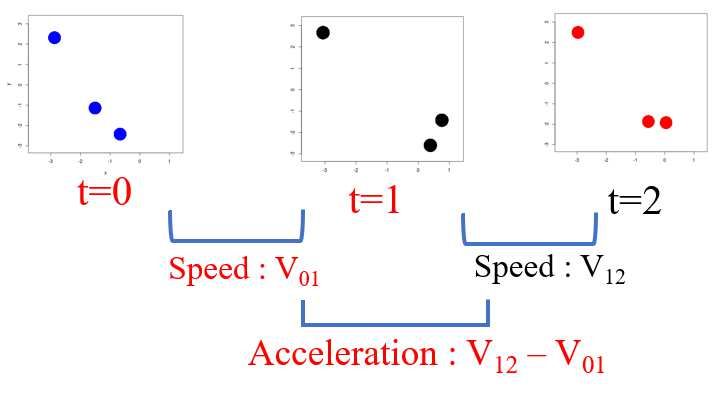
Table 1: Comparison of original 2D Sinkhorn distance and proposed 3D extension

                                      Original Sinkhorn distance               Proposed extension
 Considered time points               t, t + 1                                 t, t + 1, t + 2
 Estimated movement                   Ai → B j                                 Ai → B j → Ck
 Dimension of P and M                 2                                        3
 Element of M as cost index           ||b j − ai ||                            || (ck − b j ) − (b j − ai ) ||

cost is the distance between each pair of objects at time points t and t + 1. Cost matrix
M is the distance matrix between the objects at time point t and those at time point t + 1.
If the time is equally spaced, this distance can be thought of as a speed. Transportation
between two points is estimated using the Sinkhorn method. Transportation matrix P
and cost matrix M are both two-dimensional (2D). The optimization is described by Eq.
(1) in subsection 1. We call this situation ”speed cost”. In this case, optimal transport
matrix P represents nearest-neighbor matching.
     We assume that the objects are moving at constant velocity. Then, we calculate the
acceleration from the data obtained at three time points and use it as the cost. Table 1
shows our extension of the Sinkhorn distance from two dimensions to three dimensions.
     In summary, the proposed extension uses three time points (t, t + 1, and t + 2) rather
than two. Moreover, our estimation is not for pairs but for triples. The transportation
and cost of 2D matrices need to be extended to three-dimensional (3D) arrays. How-
ever, the optimization formula is identical. The cost is acceleration rather than speed,
or the second difference rather than the first difference. Our method returns the optimal
triples rather than pairs, and the output is 3D optimal transport array P. Therefore, we
compress the information in the triples down to pairs with the following formula and
adopt the resulting matrix as the optimal transport matrix.
                                                 n
                                      p′i j =   ∑ pi jk                                  (4)
                                                k=1

where p′i j is (i, j)th element of the compressed 2D cost matrix and pi jk is (i, j, k)th
element of original 3D cost array P. Figure 1 shows the difference between speed cost
tracking and acceleration cost tracking.

3. Simulation Analyses
To test our algorithm, we conducted three simulation analyses and compared speed cost
with acceleration cost. As mentioned, a larger value of λ leads to a wider search range.
Therefore, calculation may become difficult if λ is very large. We thus set appropriate
values (10 or 100) for each simulation. For the calculation using the original Sinkhorn
method, we used the Python Optimal Transport Library package [14].
    Initially, we generated simulation data with multiple objects that moved at constant
velocity without noise (Simulation 1). The initial coordinate values of x and y were
sampled from a normal distribution with a mean of 0 and a variance of 1. Speed along
the x and y coordinates was determined by multiplying a random number sampled from

                                                4
Fig. 1: Comparison of speed cost tracking and acceleration cost tracking. For speed
cost tracking of objects at t and t + 1, Speed V01 is used. For acceleration cost tracking
of objects at t and t + 1, Acceleration V12 − V01 is used.
this normal distribution by parameter m. Speeds of less than 0 were set to 0 to create
some objects that were at rest along the x or y coordinates. Here, m is a parameter for
adjusting speed. First, we compared the performance of tracking based on speed cost
and acceleration cost, where m = 0.5 and n = 100. Then, we changed the number of
objects n (50 or 200) and parameter m (0.5 or 2.0) to evaluate their influence.
Next, we investigated the performance obtained using a third cost array in tracking
objects moving at constant velocity (Simulation 2). We conducted two types of track-
ing, namely Acceleration (2D) and Acceleration (3D). The procedure of Acceleration
(2D) was as follows. First, the correspondence between t and t + 1 was determined
using speed cost tracking. Then, assuming constant velocity, the position at t + 2 was
predicted, and the nearest object was associated. For Acceleration (3D), the third cost
array was used, as done for Simulation 1. However, we compressed the information in
the triples down to p′ik = ∑nj=1 pi jk instead of p′i j = ∑nk=1 pi jk . The accuracy of tracking
at t + 2 was compared between Acceleration (2D) and Acceleration (3D). The param-
eter settings were m = 2.0 and n = 100.
Next, we considered random-walking objects (Simulation 3). The movement dis-
tance at each time point was sampled from the 2D normal distribution with mean vector
0 and variance matrix σ 2 I. Values of σ 2 were varied (0.1, 0.5, 1.0, 1.5, 2.0) and n was
set to 100.
Finally, we considered multiple objects that move at constant velocity with noise
(Simulation 4). The settings were the same as those for Simulation 1, where x and
y coordinate values were sampled from the normal distribution with a mean of 0 and
a variance of 1. Speed along the x and y coordinates was determined by multiplying
a random number sampled from this normal distribution by parameter m. Parameters
n and m were set to 100 and 0.5, respectively. Unlike in Simulation 1, in Simulation
3, noise was added to both x and y coordinate values each time there was movement.
The noise at each time point was sampled from the 2D normal distribution with mean
vector 0 and variance matrix σ 2 I. We used four values of σ 2 (0.01, 0.05, 0.10, 0.25).
5Fig. 2: Boxplot of performance index for 10 simulation datasets for speed cost and
acceleration cost tracking of objects moving at constant velocity without noise (Simu-
lation 1). Parameters n and m were set to 100 and 0.5, respectively. The boxes show
the lower quantile and upper quartile values of the data. The orange lines represent the
median values. The whiskers and white circle are the range of data (minimum value
to maximum value) and outlier value, respectively, which were defined by the default
settings of the matplotlib.pyplot.boxplot function in the Python library.
We evaluated the tracking performance using a performance index whose values
range between 0 and 1. Because a given object has the same index in our simulations,
the correspondence of correct answers lies diagonally in the optimal transport matrix.
Thus, the performance index is defined as the number of rows whose diagonal value is
maximum. A higher index value represents better tracking performance. In all simula-
tions, 10 datasets were generated, and the performance index was calculated for each
dataset.
3 Results
Figure 2 shows the performance index results for speed cost and acceleration cost ob-
tained with n = 100 and m = 0.5 (Simulation 1). The performance index for accelera-
tion cost was better than that for speed cost. Next, the same simulation was performed
by changing n. Figure 3 shows the performance index values obtained with n = 50 and
n = 200. For both speed cost and acceleration cost, as n increased, the performance
index decreased. Figure 4 shows the results of the same simulation with m changed
(m = 0.5 and m = 2.0) and n set to 50. For speed cost, but not for acceleration cost, the
performance index was affected by m. 2 shows the average performance index values
for each parameter setting in Simulation 1. Figure 5 shows the performance index re-
sults for Acceleration (2D) and Acceleration (3D) obtained with n = 100 and m = 2.0
(Simulation 2). Although constant-velocity motion was assumed for both cases, per-
formance was better when using the 3D cost array (Acceleration (3D)).
6Fig. 3: Boxplot of performance index for 10 simulation datasets for speed cost and
acceleration cost tracking of objects moving at constant velocity without noise (Simu-
lation 1) obtained for n = 50 and n = 200. Parameter m was set to 0.5. The description
of the objects in the boxplot is the same as Figure 2.
Fig. 4: Boxplot of performance index for 10 simulation datasets for speed cost and
acceleration cost tracking of objects moving at constant velocity without noise (Simu-
lation 1) obtained with m = 0.5 and m = 2.0. Parameter n was set to 50. The description
of the objects in the boxplot is the same as Figure 2.
7Fig. 5: Boxplot of performance index for 10 simulation datasets for tracking with ac-
celeration tracking based on 2D Sinkhorn (Acceleration (2D)) and 3D Sinkhorn (Ac-
celeration (3D)) (Simulation 2). The description of the objects in the boxplot is the
same as Figure 2.
Table 2: Average performance index for each parameter setting in Simulation 1
n m Speed cost Acceleration
cost
100 0.5 0.567 1.0
50 0.5 0.628 0.976
200 0.5 0.456 0.624
50 2 0.364 0.988
8Fig. 6: Accuracy of tracking random-walking objects (Simulation 3). The movement
distance at each time point was sampled from the 2D normal distribution with mean
vector 0 and variance matrix σ 2 I. Values of σ 2 were changed (0.1, 0.5, 1.0, 1.5, 2.0).
Parameter n was set to 100. The plots show the average performance index for 10
datasets for speed cost and 10 datasets for acceleration cost.
Figure 6 shows the results of Simulation 3. The performance index for tracking
random-walking objects was generally low for both speed cost and acceleration cost.
Figure 7 shows the results of Simulation 4. The performance index decreased as noise
increased for both speed cost and acceleration cost. The results suggest that if the
added noise is not excessively large, acceleration cost tracking outperforms speed cost
tracking. However, when the added noise is large, speed cost tracking is slightly better.
4 Discussion
For tracking an agent that is moving at constant velocity, the results of Simulation
1 show that the performance obtained using acceleration cost tracking is better and
that it is not affected by speed. Although performance deteriorates as the number of
objects increases for both tracking methods, acceleration cost tracking still shows better
performance. The results of Simulation 2 show that the Sinkhorn method with a 3D
cost array is better than that with a second cost matrix for tracking objects moving at
constant velocity. The results of Simulation 3 show that neither speed cost tracking
nor acceleration cost tracking are useful for random-walking objects. They also show
that when objects move at constant velocity, our method is superior to the nearest-
neighbor method, even if small noise is added. However, when the added noise is
large, speed cost tracking is slightly better. Thus, the above results indicate that for
objects moving at constant velocity, particularly when the movement is intense, the
number of objects is large, and the added noise is not excessively large, the proposed
method of acceleration cost tracking is superior to speed cost tracking based on the
conventional nearest-neighbor method.
9Fig. 7: Accuracy of tracking objects moving at constant velocity with noise (Simu-
lation 4). Here, σ 2 is the variance of noise. The settings are the same as those for
Simulation 1, where x and y coordinates were sampled from the normal distribution
with a mean of 0 and a variance of 1. Speed along the x and y coordinates was de-
termined by multiplying a random number sampled from the normal distribution by
parameter m. Parameters n and m were set to 100 and 0.5, respectively. The plots
show the average performance index for 10 datasets for speed cost and 10 datasets for
acceleration cost.
The advantage of using the Sinkhorn distance for tracking is that various assump-
tions regarding movement can be incorporated into cost matrix M. In this study, we
proposed a tracking method based on the assumption of uniform object motion. By
considering the third difference, the difference in acceleration, we can also express the
assumption of equal acceleration motion. In addition, if appropriate cost arrays can be
set, it may be possible to apply the proposed method to objects that move smoothly,
such as amoeba cells. Therefore, the proposed method is potentially useful for bioimag-
ing research.
Because of the flexibility of the cost matrix and cost array, the Sinkhorn method can
consider features other than motion characteristics. For example, each object in an im-
age has a specific shape. Changes in shape can be used for the cost. Moreover, multiple
costs, such as the costs of shape, distance, and acceleration, can be combined to define
an optimization cost. Our study considered just one of many potential applications of
the Sinkhorn method to the tracking problem.
5 Conclusion
We proposed a method that applies the Sinkhorn distance to track objects. We com-
pared speed cost tracking based on the conventional nearest-neighbor method and ac-
celeration cost tracking based on the proposed Sinkhorn method, and compared their
performance using simulation data. We showed that the Sinkhorn method can be ap-
10plied effectively to object tracking. Our simulation data analysis suggests that when
objects are moving at constant velocity, our method, which sets acceleration as a cost,
outperforms the traditional nearest-neighbor method in terms of tracking objects as
long as the added noise is not excessively large. To apply the proposed method to
real bioimaging data, it is necessary to set an appropriate cost indicator based on the
movement features.
6 Acknowledgement
This work was supported by Grant-in-Aid for JSPS KAKENHI Grant Number JP19J14816,
and Core Research for Evolutional Science and Technology (CREST) (grant numbers
JPMJCR1502 and JPMJCR15G1) of the Japan Science and Technology Agency (JST).
We would like to thank to the members of Matsuda Laboratory, Osaka University Grad-
uate School of Information Science, and Ishi Laboratory, Osaka University Graduate
School of Medicine, and Dr. Kazushi Mimura of Hiroshima City University for useful
advice and discussion. The authors declare no conflicts of interest.
References
[1] Katherine Celler, Gilles P van Wezel, and Joost Willemse. Single particle tracking
of dynamically localizing tata complexes in streptomyces coelicolor. Biochemical
and biophysical research communications, Vol. 438, No. 1, pp. 38–42, 2013.
[2] Auguste Genovesio, Tim Liedl, Valentina Emiliani, Wolfgang J Parak, Maité
Coppey-Moisan, and J-C Olivo-Marin. Multiple particle tracking in 3-d+ t mi-
croscopy: method and application to the tracking of endocytosed quantum dots.
IEEE Transactions on Image Processing, Vol. 15, No. 5, pp. 1062–1070, 2006.
[3] Ihor Smal, Katharina Draegestein, Niels Galjart, Wiro Niessen, and Erik Meijer-
ing. Particle filtering for multiple object tracking in dynamic fluorescence mi-
croscopy images: Application to microtubule growth analysis. IEEE transactions
on medical imaging, Vol. 27, No. 6, pp. 789–804, 2008.
[4] Nicolas Chenouard, Ihor Smal, Fabrice De Chaumont, Martin Maška, Ivo F
Sbalzarini, Yuanhao Gong, Janick Cardinale, Craig Carthel, Stefano Coraluppi,
Mark Winter, et al. Objective comparison of particle tracking methods. Nature
methods, Vol. 11, No. 3, p. 281, 2014.
[5] Yannis Kalaidzidis. Multiple objects tracking in fluorescence microscopy. Jour-
nal of mathematical biology, Vol. 58, No. 1-2, p. 57, 2009.
[6] John C Crocker and David G Grier. Methods of digital video microscopy for
colloidal studies. Journal of colloid and interface science, Vol. 179, No. 1, pp.
298–310, 1996.
11[7] Thiagalingam Kirubarajan and Yaakov Bar-Shalom. Probabilistic data associa-
tion techniques for target tracking in clutter. Proceedings of the IEEE, Vol. 92,
No. 3, pp. 536–557, 2004.
[8] Donald Reid. An algorithm for tracking multiple targets. IEEE transactions on
Automatic Control, Vol. 24, No. 6, pp. 843–854, 1979.
[9] Javier Mazzaferri, Joannie Roy, Stephane Lefrancois, and Santiago Costantino.
Adaptive settings for the nearest-neighbor particle tracking algorithm. Bioinfor-
matics, Vol. 31, No. 8, pp. 1279–1285, 2014.
[10] Marco Cuturi. Sinkhorn distances: Lightspeed computation of optimal transport.
In Advances in neural information processing systems, pp. 2292–2300, 2013.
[11] Filippo Santambrogio. Optimal transport for applied mathematicians. Birkäuser,
NY, Vol. 55, pp. 58–63, 2015.
[12] S Haker, A Tannenbaum, and A Goldstein. Optimal transport for visual tracking
and registration. In 2003 IEEE International Workshop on Workload Characteri-
zation (IEEE Cat. No. 03EX775), Vol. 1, pp. 265–269, 2003.
[13] Cédric Villani. Optimal transport: old and new, Vol. 338. Springer Science &
Business Media, 2008.
[14] Rémi Flamary and Nicolas Courty. Pot: Python optimal transport library, 2017.
12You can also read