LOW-COST FPGAS ACCELERATING ODE-BASED NEURAL NETWORKS ON
←
→
Page content transcription
If your browser does not render page correctly, please read the page content below
ACCELERATING ODE-BASED N EURAL N ETWORKS ON
                                                               L OW-C OST FPGA S

                                                                                              A P REPRINT
arXiv:2012.15465v3 [cs.LG] 29 Mar 2021

                                                            Hirohisa Watanabe                                         Hiroki Matsutani
                                                              Keio University                                          Keio University
                                                3-14-1 Hiyoshi, Kohoku-ku, Yokohama, Japan               3-14-1 Hiyoshi, Kohoku-ku, Yokohama, Japan
                                                     watanabe@arc.ics.keio.ac.jp                              matutani@arc.ics.keio.ac.jp

                                                                                            March 30, 2021

                                                                                             A BSTRACT
                                                  ODENet is a deep neural network architecture in which a stacking structure of ResNet is imple-
                                                  mented with an ordinary differential equation (ODE) solver. It can reduce the number of parameters
                                                  and strike a balance between accuracy and performance by selecting a proper solver. It is also possi-
                                                  ble to improve the accuracy while keeping the same number of parameters on resource-limited edge
                                                  devices. In this paper, using Euler method as an ODE solver, a part of ODENet is implemented as
                                                  a dedicated logic on a low-cost FPGA (Field-Programmable Gate Array) board, such as PYNQ-Z2
                                                  board. As ODENet variants, reduced ODENets (rODENets) each of which heavily uses a part of
                                                  ODENet layers and reduces/eliminates some layers differently are proposed and analyzed for low-
                                                  cost FPGA implementation. They are evaluated in terms of parameter size, accuracy, execution
                                                  time, and resource utilization on the FPGA. The results show that an overall execution time of an rO-
                                                  DENet variant is improved by up to 2.66 times compared to a pure software execution while keeping
                                                  a comparable accuracy to the original ODENet.

                                         Keywords Neural network · CNN · ODE · Neural ODE · FPGA

                                         1 Introduction

                                         ResNet [1] is a well-known deep neural network (DNN) architecture with high accuracy. In addition to conventional
                                         forward propagation of DNNs, it has shortcut or skip connections that directly add the input of a layer to the output of
                                         the layer. Since it can mitigate vanishing and exploding gradient problems, we can stack more layers to improve pre-
                                         diction accuracy. However, stacking many layers increases the number of parameters of DNNs; in this case, memory
                                         requirement becomes severe in resource-limited edge devices.
                                         ODENet [2] that employs an ordinary differential equation (ODE) solver in DNNs was proposed to reduce weight
                                         parameters of the network. Stacking structure of layers in ResNet can be represented with an ODE solver, such as
                                         Euler method. ODENet thus uses an ODE solver in prediction and training processes so that M layers in ResNet
                                         are replaced with M repeated executions of a single layer, as shown in Figures 1 and 2. In this case, ODENet can
                                         significantly reduce the number of parameters compared to the original ResNet while keeping the equivalent prediction
                                         and training processes.
                                         Field-Programmable Gate Array (FPGA) is an energy-efficient solution, and it has been widely used in edge devices
                                         for machine learning applications. In this paper, we thus propose an FPGA-based acceleration of ODENet. A core
                                         component of ODENet, called ODEBlock, that consists of convolution layers, batch normalization [3], and activation
                                         function is implemented on a programmable logic of low-cost FPGA board, such as PYNQ-Z2 board. Our contribution
                                         is that, as ODENet variants, reduced ODENets (rODENets) each of which heavily uses a part of ODEBlocks and
                                         reduces/eliminates some layers differently are proposed and analyzed for low-cost FPGA implementation. They are
                                         evaluated in terms of parameter size, accuracy, execution time, and resource utilization on the FPGA.
Accelerating ODE-Based Neural Networks on Low-Cost FPGAs                         A PREPRINT

                                                                                Figure 2: ODENet architecture
                Figure 1: ResNet architecture

Many studies on FPGA-based DNN accelerators have been reported. In [4], such accelerators and their techniques,
such as binarization and quantization, are surveyed. When a quantization using 2-bit weight parameters is applied to
ResNet-18, 10.3% accuracy loss is reported. In [5], circuit techniques that minimize information loss from quantization
are proposed and applied to ResNet-18 and 50. In [6], ResNet-50 and 152 are implemented on Intel Arria-10 FPGA
using a 16-bit format and external memories. Microsoft Brainwave platform supports ResNet-50 [7]. Please note that
this work focuses on low-cost FPGA platforms, such as PYNQ-Z2. Also our approach is orthogonal to quantization
techniques and can be combined with for further reducing the parameter sizes.
The rest of this paper is organized as follows. Section 2 provides a brief review of basic technologies about ODENet.
Section 3 implements a building block of ODENet on the FPGA, and Section 4 shows the evaluation results. Section
5 concludes this paper.

2 Preliminaries

2.1 ResNet

In neural networks that serially stack many layers, training process may be prevented when gradients become vanish-
ingly small in one of the layers (i.e., vanishing gradient problem). Also, there may be a possibility that the training
becomes unstable when gradient descent is diverging (i.e., exploding gradient problem). ResNet [1] was proposed
to address these issues and improve the prediction accuracy by introducing shortcut connections that enable to stack
many layers. Figure 1 illustrates ResNet architecture. As shown in the figure, ResNet consists of a lot of building
blocks. Each building block receives input data zt and executes 3 × 3 convolution, batch normalization [3], ReLU [8]
as an activation function, 3 × 3 convolution, and batch normalization. For example, ResNet architecture, which will be
shown in Table 4, can be used in image classification tasks, such as CIFAR-10 and CIFAR-100 datasets. In this paper,
building blocks executing the same computations are grouped as layerx, where x = 1, 2, 3. ResNet size is denoted as
ResNet-N, where N is the total number of convolution and fully-connected steps in the building blocks including the
pre- and post-processing layers.
Let z ∈ RZ and y ∈ RZ be an input and an output of ResNet, respectively. A network parameter θ is interpreted as a
mapping function H : z → y. Assuming a normal forward propagation, an output of a building block is represented
as a function f (z, θ). When an input of a building block is additionally added to an output of the building block with a
shortcut connection, the function is changed to f (z, θ) + z. Even with a shortcut connection, an output of the building
block itself is still H(z). Thus, its residual should be trained in the training process so that f (z, θ) = H(z) − z. In
this case, a gradient at least contains 1; thus, vanishing gradient problem can be mitigated.
Assuming ResNet consists of multiple building blocks, an input to the (t + 1)-th building block is represented as
follows.
                                                zt+1 = zt + f (zt , θt ),                                            (1)
where zt and θt denote the input and parameter of the t-th building block, respectively.

                                                           2
Accelerating ODE-Based Neural Networks on Low-Cost FPGAs A PREPRINT
2.2 Ordinary Differential Equation
ODE is an equation containing functions of one variable and their derivatives. For example, a first-order differential
equation is represented as follows.
dz
= f (z(t), t, θ), (2)
dt
where f and θ represent dynamics and the other parameters, respectively. Assuming f is known and z(t0 ) is given, a
problem to find z(t1 ) that satisfies the above equation is known as an initial value problem. It is formulated as follows.
Z t1
z(t1 ) = z(t0 ) + f (z(t), t, θ)dt (3)
t0
= ODESolve(z(t0 ), t0 , t1 , f ) (4)
In the right side of Equation 3, the second term contains an integral of a given function. It cannot be solved analytically
for arbitrary functions, so a numerical approximation is typically employed to solve Equation 3. To solve the equation,
ODESolve function is defined as shown in Equation 4. In ODESolve function, integration range [t0 , t1 ] is divided into
partitions with step size h. For t0 < · · · ti < · · · t1 , it computes corresponding zi using a recurrence formula. As a
method to compute z(t1 ) in Equation 4, well-known ODE solvers, such as Euler method, second-order Runge-Kutta
method, and fourth-order Runge-Kutta method, can be used [9]. They can approximately solve Equation 3 in the
first-order, second-order, and fourth-order accuracy, respectively. Below is Euler method.
z(ti+1 ) = z(ti ) + hf (z(ti ), ti , θ) (5)
2.3 ODENet
An output of building blocks in ResNet can be computed with a recurrence formula, as shown in Equation 1. Please
note that Equation 1 is similar to Equation 5 except that the former basically assumes vector values while the latter
assumes scalar values. Thus, one building block is interpreted as one step in Euler method. As mentioned in Section
2.2, since Euler method is a first-order approximation of Equation 3, an output of ResNet building block can be
interpreted as well. Since Equation 3 can be solved by Equation 4, the output of ResNet can be solved by the same
equation. Here, a building block of ResNet is replaced with an ODEBlock using ODESolve function. Neural network
architecture consisting of such ODEBlocks is called ODENet. Figure 2 shows an ODENet architecture. ODENet that
repeats the same ODEBlock M times is interpreted as ResNet that implements M building blocks.
Prediction tasks of ODENet are executed based on Equation 4. In training process, it is required that gradients are
back-propagated along neural network layers via ODESolve function. To compute the gradients, ODENet uses an
adjoint method [10] in the training process. Here, loss function L of ODENet is represented as follows.
L(z(t1 )) = L(ODESolve(z(t0 ), t0 , t1 , f )) (6)
∂L
Let an adjoint vector a be a = ∂z(t) . The following equation is satisfied with respect to a.
da(t) ∂f (z(t), t, θ)
= −a⊤ (7)
dt ∂z(t)
Based on Equations 7 and 4, a gradient of parameter θ derived by a loss function is computed as follows.
Z t0
dL ∂f (z(t), t, θ)
=− a(t)⊤ dt
dθ t1 ∂θ
(8)
⊤ ∂f (z(t), t, θ)
= ODESolve 0, t1 , t0 , −a(t)
∂θ
z(t) and a(t) can be computed with ODESolve function. A training function can be summarized as follows by using
Equation 8 and these values [2].
z(t0 ) = ODESolve(z(t1 ), t1 , t0 , f (z(t), t, θ))
∂f (z(t), t, θ
a(t0 ) = ODESolve a(t1 ), t1 , t0 , −a(t)⊤
∂z(t) (9)
dL ∂f (z(t), t, θ)
= ODESolve 0, t1 , t0 , −a(t)⊤
dθ ∂θ
3Accelerating ODE-Based Neural Networks on Low-Cost FPGAs A PREPRINT
Figure 3: ODEBlock design on FPGA
Please note that vector size of 0 in Equation 9 is same as that of θ. In the original Equation 8, it is necessary to
compute a(t) and z(t) for each t. On the other hand, in the case of Equation 9, z(t) is computed first using ODESolve
function; then a(t) is computed based on z(t), and the gradient is computed based on z(t) and a(t). Thus, the gradient
is computed sequentially without keeping a(t) and z(t) for each t, so memory usage can be reduced as well. Based on
the above-mentioned properties of ODENet, the benefit against the original ResNet is that the number of parameters
can be reduced by ODENet. In the prediction process, ResNet is represented with M different building blocks, while
ODENet repeatedly uses a single ODEBlock M times. When the number of parameters for one building block is
O(L), those of ResNet and ODENet are O(LM ) and O(L), respectively. As we will see in Table 2, the number of
parameters for pre- and post-processing layers (e.g., conv1 and fc) is not significant, it is expected that the number
1
of parameters of ResNet is reduced to approximately M . In other words, different parameters are used for each t
in ResNet, as shown in Equation 1. In ODENet, on the other hand, as shown in Equation 2, θ is independent of t;
thus, it can be trained while the parameters are fixed irrespective of t. Please note that different ODE solvers can be
used in prediction and training processes. For example, a fourth-order Runge-Kutta method is used for training with
high accuracy, while Euler method is used for prediction tasks for low latency and simplicity. We can strike a balance
between accuracy and performance by selecting a proper solver.
3 FPGA Implementation
3.1 ODEBlock
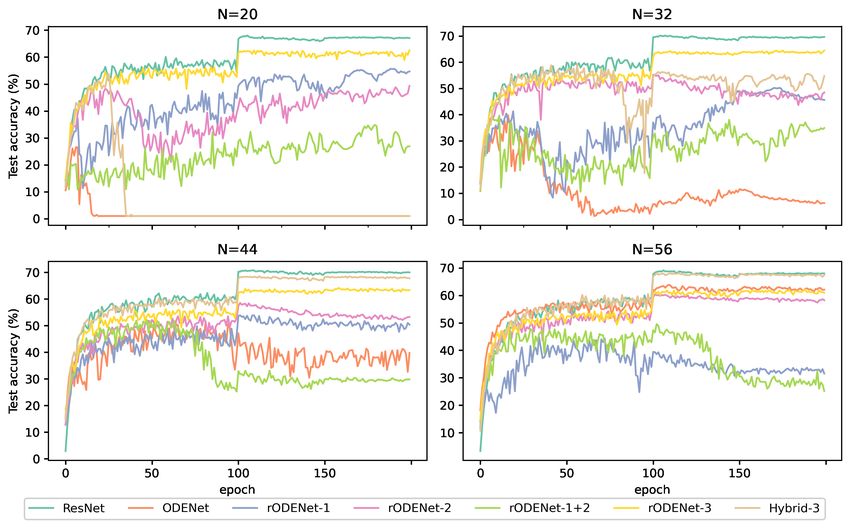
In this paper, as a target platform, we employ SoC type FPGA devices that integrate programmable logic (PL) part and
processor (PS) part, as shown in Figure 3. PS part consists of CPU and DRAM, while PL part has programmable logic.
We use TUL PYNQ-Z2 board [11] in this paper. Figure 4 shows the FPGA board, and Table 1 shows the specification.
As shown in Figure 3, a part of the ODEBlock is implemented on PL part as a dedicated circuit, while the others are
executed on PS part as software.
Table 1: Specification of PYNQ-Z2 board
OS PYNQ Linux (Ubuntu 18.04)
CPU ARM Cortex-A9 @ 650MHz × 2
DRAM 512MB (DDR3)
FPGA Xilinx Zynq XC7Z020-1CLG400C
Figure 4: Overview of PYNQ-Z2 board
4Accelerating ODE-Based Neural Networks on Low-Cost FPGAs A PREPRINT
Table 2: Network structure of ODENet
Layer Output size Detail Parameter size [kB] # of executions per block
conv1 32 × 32, 16ch 3 × 3,stride 1 1.86 1
3×3 N −2
layer1 32 × 32, 16ch , stride 1 19.84
3×3 6
3×3
layer2_1 16 × 16, 32ch , stride 2 55.81 1
3×3
3×3 N −8
layer2_2 16 × 16, 32ch , stride 1 76.54
3×3 6
3×3
layer3_1 8 × 8, 64ch , stride 2 222.21 1
3×3
3×3 N −8
layer3_2 8 × 8, 64ch , stride 1 300.54
3×3 6
Average pooling,
fc 1 × 100 26.00 1
100d fc, softmax
Table 2 shows network structure of ODENet with a given N. It consists of several building blocks or “layers” as shown
in the table: conv1, input1, input2_1, input2_2, input3_1, input3_2, and fc. In the case of ODENet, only a single
block instance is implemented for each layer, and the same instance is continuously executed instead. For example,
the numbers of executions per block for input1, input2_2, and input3_2 are N6−2 , N6−8 , and N 6−8 , respectively; the
others are executed only once. In this paper, we thus implement input1, input2_2, and input3_2 individually on a
resource-limited FPGA board. That is, each of these layers is implemented on PL part of PYNQ-Z2, while the other
parts are executed on PS part as software. Euler method is used as an ODE solver.
Each layer consists of five steps: 1) convolution, 2) batch normalization, 3) activation function (ReLU), 4) convolution,
and 5) batch normalization. The convolution step differs in each layer. That is, the input/output channel numbers for
layer1, layer2_2, and layer3_2 are 16, 32, and 64. The input/output feature map sizes for layer1, layer2_2, and
layer3_2 are 8×8, 16×16, and 32×32. Their kernel size is 3×3 and stride width is 1. The above mentioned five
steps are implemented in Verilog HDL. 32-bit Q20 fixed-point number format is used. Multiply-add units are used
in the convolution and ReLU steps, and multiply-add units, division unit, and square root unit are used in the batch
normalization steps for computing mean, variance, and standard deviation. Weight parameters θ of the two convolution
steps are stored in Block RAM (BRAM) of the FPGA. Input and output feature maps for all the channels are also stored
in the BRAM.
Most of computation time is consumed in the convolution steps 1 . Our convolution and ReLU step implementations
are scalable; that is, we can increase the number of multiply-add units from 1 to 64 depending on available resources
but it is also restricted by the number of output channels. Their execution cycles (except for the batch normalization)
decrease in inverse proportion to the number of multiply-add units. We implemented layer1, layer2_2, and layer3_2
each using 1, 4, 8, 16, and 32 multiply-add units. They are referred to as conv_x1, conv_x4, conv_x8, conv_x16,
and conv_x32, respectively. For example, their execution cycles of layer3_2 are 23.78M, 6.07M, 3.12M, 1.64M, and
0.90M cycles, respectively. In these implementations, since only conv_x32 could not satisfy a timing constraint of our
target FPGA board (i.e., 100MHz), we mainly use conv_x16 in this paper.
3.2 Resource Utilization
Table 3 shows resource utilizations of layer1, layer2_2, and layer3_2 implemented on PL part of the FPGA for ODENet
and its variants in this paper. Here, we show the result when n multiply-add units are used for the convolution and
ReLU steps. They are denoted as conv_xn implementations. As shown in the table, if we implement layer3_2 on
PL part of the FPGA, BRAM utilization becomes 100%. In this case, the utilizations of DSP, LUT, and FF still have
room and can implement some other application logic, but we cannot implement more weight parameters or larger
feature maps without relying on external DRAMs. On the other hand, BRAM utilizations of layer1 and layer2_2 are
not as high as layer3_2, and the other resources also have enough room, so we can implement both the layers on PL
part of the FPGA. In the next section, we can thus consider four cases: 1) only layer1 is implemented on PL part, 2)
only layer2_2 is implemented on PL part, 3) layer1 and layer2_2 are implemented on PL part, and 4) only layer3_2 is
implemented on PL part of the FPGA.
1
The two convolution steps consume about 99% of execution cycles of layer3_2 when only a single multiply-add unit is used in
our implementation.
5Accelerating ODE-Based Neural Networks on Low-Cost FPGAs A PREPRINT
Table 3: Resource utilizations of layer1, layer2_2, and layer3_2 on Zynq XC7Z020
Layer Parallelism BRAM DSP LUT FF
conv_1 56 (40.00%) 8 (3.63%) 1486 (2.79%) 835 (0.78%)
conv_4 56 (40.00%) 20 (9.09%) 2992 (5.62%) 1358 (1.28%)
layer1
conv_8 56 (40.00%) 36 (16.36%) 4740 (8.91%) 2058 (1.93%)
conv_16 64 (45.71%) 68 (30.91%) 8994 (16.91%) 4145 (3.90%)
conv_1 56 (40.00%) 8 (3.63%) 1482 (2.79%) 833 (0.78%)
conv_4 56 (40.00%) 20 (9.09%) 2946 (5.53%) 1346 (1.27%)
layer2_2
conv_8 56 (40.00%) 36 (16.36%) 4737 (8.90%) 2032 (1.91%)
conv_16 56 (40.00%) 68 (30.91%) 8844 (16.62%) 4873 (4.58%)
conv_1 140 (100.00%) 8 (3.63%) 1692 (3.18%) 927 (0.87%)
conv_4 140 (100.00%) 20 (9.09%) 3048 (5.73%) 1411 (1.33%)
layer3_2
conv_8 140 (100.00%) 36 (16.36%) 4907 (9.22%) 2059 (1.94%)
conv_16 140 (100.00%) 68 (30.91%) 12720 (23.91%) 6378 (5.99%)
4 Evaluations
CIFAR-100 is used as a dataset in this paper. ODENet on the FPGA is evaluated in terms of the number of parameters,
accuracy, and execution time when a part of convolution layers is executed by PL part.
4.1 Network Configuration
Here, we introduce reduced ODENet (rODENet) variants for low-cost FPGA implementation. As shown in Table 4,
seven network architectures including our rODENet variants listed below are used in this evaluation. Please note that
the number of stacked blocks means the number of block instances implemented, while the number of executions per
block means the number of iterations on the same block instance.
• ResNet-N: Baseline ResNet
• ODENet-N: layer1, layer2_2, and layer3_2 in ResNet-N are replaced with corresponding ODEBlocks.
• rODENet-1-N: layer2_2 and layer3_2 are removed. layer1 is replaced with ODEBlock, and the number
of executions on layer1 is increased instead so that the total execution count of building blocks is same as
ResNet-N.
• rODENet-2-N: The number of executions on layer1 is reduced to 1 and layer3_2 is removed. layer2_2 is
replaced with ODEBlock, and the number of executions on layer2_2 is increased instead.
• rODENet-1+2-N: layer3_2 is removed. layer1 and layer2_2 are replaced with ODEBlocks, and the numbers
of executions on layer1 and layer2_2 are increased instead.
• rODENet-3-N: The number of executions on layer1 is reduced to 1 and layer2_2 is removed. layer3_2 is
replaced with ODEBlock, and the number of executions on layer3_2 is increased instead.
• Hybrid-3-N: Only layer3_2 in ResNet-N is replaced with ODEBlock. The other layers are the same as those
in ResNet.
We can expect that a computation of ODENet-N is compatible with that in ResNet-N. On the other hand, our
rODENet-1-N, rODENet-2-N, rODENet-1+2-N, and rODENet-3-N execute the same number of building blocks
as ResNet-N, but they heavily use layer1, layer2_2, layer1 and layer2_2, and layer3_2, respectively. Our intention
is that these heavily-used layers are offloaded to PL part as shown in Figure 3. In addition, Hybrid-3-N, which is a
middle of ResNet-N and ODENet-N, is evaluated as a high-accuracy variant.
Euler method is used as an ODE solver, because it is simple and requires only a small temporary memory at prediction
time. In Table 4, conv1 is the pre-processing step that executes 3×3 convolution, batch normalization, and ReLU as
an activation function. Then, various building blocks (e.g., layer1 to layer3_2 in Table 4) are executed as shown in
Figure 1. Finally, fc is the post-processing step that executes global average pooling, fully-connected layer to all the
output classes, and Softmax as an activation function. Stride width is set to 1 in most of building blocks except for
layer2_1 and layer3_1, in which stride width is set to 2 in order to reduce the output feature map size.
4.2 Parameter Size
Figure 5 shows the total parameter size for each architecture listed in Section 4.1, assuming that each parameter is
implemented in a 32-bit format.
6Accelerating ODE-Based Neural Networks on Low-Cost FPGAs A PREPRINT
Table 4: Network structure of ResNet, ODENet, and rODENet variants
# of stacked blocks / # of executions per block
Layer
ResNet ODENet rODENet-1 rODENet-2 rODENet-1+2 rODENet-3 Hybrid-3
conv1 1/1 1/1 1/1 1/1 1/1 1/1 1/1
N −2
layer1 6 /1 1 / N6−2 1 / N2−6 1/1 1 / N 4−4 1/1 N −2
6 /1
layer2_1 1/1 1/1 1/1 1/1 1/1 1/1 1/1
N −8
layer2_2 6 /1 1 / N6−8 0/0 1 / N2−8 1 / N 4−8 0/0 N −8
6 /1
layer3_1 1/1 1/1 1/1 1/1 1/1 1/1 1/1
N −8
layer3_2 6 /1 1 / N6−8 0/0 0/0 0 /0 1 / N2−8 1 / N 6−8
fc 1/1 1/1 1/1 1/1 1/1 1/1 1/1
Figure 5: Parameter size of ResNet, ODENet, and rODENet variants
As shown in Table 5, parameter size of ResNet-N is proportional to the number of stacked building blocks (see Figure
1). Please note that parameter sizes of ODENet-N and the rODENet variants are independent of N, since the number
of stacked instances is independent of N (see Figure 2). In the rODENet variants, their parameter sizes depend on
layers actually implemented. When N is 20 (the smallest case), parameter sizes of ODENet-N and rODENet-3 are
36.24% and 43.29% less than that of ResNet-20, respectively. When N is 56 (the largest case), their parameter sizes
are 79.54% and 81.80% less than that of ResNet-56, respectively. Although structure of Hybrid-3-N is similar to that
of ResNet-N except for layer3_2, it can reduce the parameter size by 26.43% and 60.16% compared to ResNet-N
when N is 20 and 56, respectively. Please note that the parameter size reduction by using ODEBlock is independent
of the other parameter reduction techniques, such as quantization [4], and can be incorporated with them to further
reduce the parameter size.
4.3 Accuracy
In this experiment, SGD [12] is used as an optimization function. As L2 regularization, 1 × 10⁻⁴ is added to each
layer. For the training process, the number of epochs is 200. The learning rate is started with 0.01, and it is reduced
1
by 10 when the epoch becomes 100 and 150.
Figure 6 shows the evaluation results of accuracy in the seven network architectures listed in Table 4. As shown in
the graphs, when N is 20, the training results are unstable especially in ODENet-N and Hybrid-3-N. When N is 56,
on the other hand, accuracies of most architectures are improved and become stable, except for rODENet-1-N and
rODENet-1+2-N. Among the rODENet variants, rODENet-3 is stable and shows relatively high accuracy when N is
20, 32, 44, and 56; thus we mainly focus on rODENet-3.
7Accelerating ODE-Based Neural Networks on Low-Cost FPGAs A PREPRINT
Figure 6: Accuracy of four network architectures when N={20,32,44,56}
In Hybrid-3-N, the accuracy is the almost same as ResNet-N when N is 44 and 56. More specifically, accuracies
of ResNet-44 and Hybrid-3-44 are 70.74% and 68.58%, and those of ResNet-56 and Hybrid-3-56 are 69.09% and
68.11%; thus there is up to 2.16% accuracy loss. The accuracy difference between ResNet-44 and ResNet-56 is 1.65%,
while that of Hybrid-3-44 and Hybrid-3-56 is only 0.47%; thus, they are robust against overfitting (i.e., degradation
of generalization ability) due to larger N.
In rODENet-3-N, the accuracy is the second highest next to that of ResNet-N when N is 20 and 32. Accuracies of
ResNet-20 and rODENet-3-20 are 68.02% and 62.54%, and the accuracy difference is 5.48%. Those of ResNet-32
and rODENet-3-32 are 70.16% and 64.46%, and the difference is 5.70%. These differences are large compared to
those of Hybrid-3-N when N is 44 and 56. Still, rODENet-3-N is stable for all the sizes, which means that this
architecture has the highest robustness against increasing N among the rODENet variants. Because of its stability, we
can use rODENet-3-N even if the optimal network architecture is not known yet.
In ODENet-N, the accuracy is relatively high next to those of ResNet-N and Hybrid-3-N when N is 56. However, it
is unstable when N is small. The reason for this unstability is that the step size was relatively large and thus it could
not acquire the dynamics sufficiently. In ODENet and its variants, it is interpreted that connections of ResNet layers
are continuous. It is pointed out that there may be a possibility that ODENet cannot compute the gradients accurately
[13]. This may be one reason for the unstability when N is small.
In summary, our rODENet-3 is stable and shows relatively high accuracy for all the sizes in our experiment. Consid-
ering the parameter size, it can strike a balance between the parameter size reduction, stability, and accuracy.
4.4 Execution Time
The ODENet variants implemented on the FPGA mentioned in Section 3 are evaluated in terms of prediction time.
More specifically, the following architectures are compared.
• ResNet-N: In ResNet-N, all the layers are executed on PS part as software.
• rODENet-*-N: In the rODENet variants, only heavily-used layers are offloaded to PL part as dedicated
circuits. The other layers are software. Among rODENet variants, we mainly focus on rODENet-3-N since
8Accelerating ODE-Based Neural Networks on Low-Cost FPGAs A PREPRINT
Table 5: Execution time of ResNet, ODENet, and rODENet variants (PS: Cortex-A9 @650MHz, PL: @100MHz)
Offload Total w/o Target w/o Ratio of Target w/ Total w/ Overall
Model N
target PL [s] PL [s] target [%] PL [s] PL [s] speedup
20 0.54 – – – – –
32 0.89 – – – – –
ResNet –
44 1.24 – – – – –
56 1.58 – – – – –
20 0.57 0.44 76.89 0.15 0.28 1.99
32 0.94 0.81 86.06 0.29 0.42 2.26
rODENet-1 layer1
44 1.30 1.17 89.91 0.42 0.55 2.37
56 1.67 1.54 92.14 0.55 0.68 2.45
20 0.52 0.33 63.82 0.11 0.30 1.75
32 0.86 0.67 77.74 0.22 0.41 2.08
rODENet-2 layer2_2
44 1.19 1.00 84.14 0.33 0.52 2.28
56 1.52 1.33 87.46 0.44 0.63 2.40
20 0.55 0.25 / 0.17 44.98 / 31.09 0.09 / 0.06 0.27 1.99
32 layer1 / 0.89 0.42 / 0.33 47.54 / 37.71 0.15 / 0.11 0.39 2.24
rODENet-1+2
44 layer2_2 1.23 0.60 / 0.50 48.63 / 40.75 0.22 / 0.17 0.52 2.38
56 1.60 0.81 / 0.66 50.40 / 41.45 0.29 / 0.22 0.64 2.52
20 0.54 0.35 64.48 0.10 0.29 1.85
32 0.88 0.69 78.44 0.20 0.39 2.26
rODENet-3 layer3_2
44 1.23 1.04 84.44 0.30 0.49 2.50
56 1.57 1.38 87.87 0.40 0.59 2.66
20 0.56 0.12 21.24 0.03 0.47 1.18
32 0.90 0.23 25.83 0.07 0.74 1.23
ODENet-3 layer3_2
44 1.25 0.34 27.67 0.10 1.00 1.24
56 1.60 0.46 28.98 0.13 1.27 1.26
20 0.53 0.12 22.38 0.03 0.44 1.19
32 0.88 0.23 26.65 0.07 0.71 1.24
Hybrid-3 layer3_2
44 1.23 0.35 28.11 0.10 0.99 1.25
56 1.56 0.46 29.64 0.13 1.23 1.27
it is advantageous in terms of the parameter size and accuracy. In this case, layer3_2 is PL part and the others
are PS part.
• ODENet-3-N: In ODENet-N, layer3_2 is PL part and the others are PS part.
• Hybrid-3-N: In Hybrid-3-N, layer3_2 is PL part and the others are PS part.
An image size in CIFAR-100 dataset is (channel, height, width) = (3, 32, 32), and prediction time for each image is
measured. As an FPGA platform, TUL PYNQ-Z2 board that integrates PS and PL parts is used in this experiment.
As listed in Table 1, in PS part, two ARM Cortex-A9 processors are running at 650MHz. In PL part, the operating
frequency of the dedicated circuits is 100MHz. Vivado 2017.2 was used for the design synthesis and implementation of
the ODEBlocks (i.e., layer1, layer2_2, and layer3_2) implemented on PL part. We employ conv_x16 implementation
that uses 16 multiply-add units for the convolution and ReLU steps. PS and PL parts are typically connected via AXI
bus and DMA transfer is used for their communication though not fully implemented in our design. We assume that
data transfer latency between PS and PL parts is 1 cycle per float32. This is an optimistic assumption, but we use this
value for simplicity because it varies depending on an underlying hardware platform.
Table 5 shows the execution times and speedup rates of the seven architectures mentioned above when they are imple-
mented on the FPGA board. In this table, “Offload target” means layer(s) implemented on PL part of the FPGA. For
example, the offloaded target is layer3_2 in rODENet-3-N, ODENet-3-N, and Hybrid-3-N. As shown in the table,
execution time of layer3_2 takes up only 21.24% to 29.64% of total execution time of ODENet-3-N and Hybrid-3-N.
On the other hand, layer3_2 is heavily used intentionally in rODENet-3-N, and its execution time takes up 64.48% to
87.87%. Thus, by offloading layer3_2 to PL part, the total execution time of rODENet-3-N is 2.66 times faster than a
pure software execution when N is 56, which is the largest overall speedup by the FPGA.
Regarding Hybrid-3-N and ODENet-3-N, the overall speedup by the FPGA for Hybrid-3-N is equal to or higher than
that of ODENet-3-N in all the sizes. This is because the ratio of layer3_2 in Hybrid-3-N is slightly higher than that
in ODENet-3-N and the speedup rate of only layer3_2 by the FPGA is almost constant regardless of N.
9Accelerating ODE-Based Neural Networks on Low-Cost FPGAs A PREPRINT
In summary, the overall speedup rate by the FPGA is relatively high in the rODENet variants, followed by Hybrid-3-N
and ODENet-3-N. Although all the rODENet variants show favorable speedup, only rODENet-3-N shows high and
stable accuracy, as shown in Section 4.3. Regarding the overall speedup compared to the original ResNet, rODENet-
3-56 is 2.67 times faster than a pure software execution of ResNet-56. Although the overall speedup by the FPGA
is smallest in Hybrid-3-20, it is still 1.22 times faster than a software execution of ResNet-20. Please note that, as
mentioned in Section 4.3, the accuracy of rODENet-3-N is quite high and stable when N is 20 and 32. When N
is 44 and 56, its accuracy is less than Hybrid-3-N, but it is still comparable to ODENet-3-N. Thus, our proposed
rODENet-3-N would be a practical choice in terms of the parameter size, accuracy, stability, and execution time 2 .
5 Summary
To offload a part of ResBlock building blocks on PL part of low-cost FPGA devices, in this paper we focused on
ODENet and it was redesigned. More specifically, as ODENet variants, reduced ODENets (rODENets) each of which
heavily uses a part of ODEBlocks and reduces some layers differently were proposed and analyzed for low-cost FPGA
devices. We examined seven network architectures including the original ResNet (ResNet-N), the original ODENet
(ODENet-N), and our proposed rODENet variants (e.g., rODENet-3-N) in terms of the parameter size, accuracy, and
execution time. A part of ODEBlocks, such as layer1, layer2_2, and layer3_2, was implemented on PL part of PYNQ-
Z2 board to evaluate their FPGA resource utilization. For example, rODENet-3-N heavily uses layer3_2, reduces
layer1, eliminates layer2_2, and offloads layer3_2 to PL part of the FPGA.
The evaluation results using CIFAR-100 dataset showed that the parameter sizes of rODENet-3-N are 43.29% and
81.80% less than those of ResNet-N when N is 20 and 56, respectively. The accuracies of rODENet-3-N are the
second highest next to that of ResNet-N when N is 20 and 32. When N is 44 and 56, its accuracy is less than Hybrid-
3-N, but it is still comparable to ODENet-3-N. rODENet-3-N is 2.66 times faster than a pure software execution
when N is 56, which is the largest overall speedup by the FPGA. It is 2.67 times faster than a software execution of
ResNet-N when N is 56. In summary, our proposed rODENet-3-N can strike a balance between the parameter size,
accuracy, stability, and execution time.
As a future work, we are working on the accuracy loss issue when the adjoint method is used for training process.
Further experiments using more accurate ODE solvers, such as Runge-Kutta method, are necessary. Lastly, we are
planning to offload the training process of the rODENet variants to FPGA devices.
References
[1] K. He, X. Zhang, S. Ren, and J. Sun, “Deep Residual Learning for Image Recognition,” in Proceedings of the
IEEE Conference on Computer Vision and Pattern Recognition (CVPR’16), Jun 2016, pp. 770–778.
[2] R. T. Q. Chen, Y. Rubanova, J. Bettencourt, and D. Duvenaud, “Neural Ordinary Differential Equations,” in
Proceedings of the Annual Conference on Neural Information Processing Systems (NeuroIPS’18), Dec 2018, pp.
6572–6583.
[3] S. Ioffe and C. Szegedy, “Batch Normalization: Accelerating Deep Network Training by Reducing Internal
Covariate Shift,” in Proceedings of the International Conference on Machine Learning (ICML’15), Jul 2015, pp.
448–456.
[4] K. Guo, S. Zeng, J. Yu, Y. Wang, and H. Yang, “A Survey of FPGA-Based Neural Network Accelerator,”
arXiv:1712.08934v3, Dec 2018.
[5] J. Faraone, M. Kumm, M. Hardieck, P. Zipf, X. Liu, D. Boland, and P. H. Leong, “AddNet: Deep Neural Net-
works Using FPGA-Optimized Multipliers,” IEEE Transactions on Very Large Scale Integration (VLSI) Systems,
vol. 28, no. 1, pp. 115–128, Jan 2020.
[6] Y. Ma, M. Kim, Y. Cao, S. Vrudhula, and J. sun Seo, “End-to-End Scalable FPGA Accelerator for Deep Residual
Networks,” in Proceedings of the International Symposium on Circuits and Systems (ISCAS’17), May 2017, pp.
1–4.
[7] J. Duarte et al., “FPGA-Accelerated Machine Learning Inference as a Service for Particle Physics Computing,”
Computing and Software for Big Science, vol. 3, no. 13, Oct 2019.
2
Performance improvement is still modest since some layers are executed by software. It would be further improved if weight
parameters of more layers can be stored in BRAM. Although we used 32-bit fixed-point numbers, using reduced bit widths (e.g.,
16-bit or less) can implement more layers in PL part.
10Accelerating ODE-Based Neural Networks on Low-Cost FPGAs A PREPRINT
[8] V. Nair and G. E. Hinton, “Rectified Linear Units Improve Restricted Boltzmann Machines,” in Proceedings of
the International Conference on Machine Learning (ICML’10), Jun 2010, pp. 807–814.
[9] W. H. Press, S. A. Teukolsky, W. T. Vetterling, and B. P. Flannery, Numerical Recipes. The Art of Scientific
Computing, 3rd Edition. Cambridge University Press, 2007.
[10] L. S. Pontryagin, V. G. Boltyanskii, R. V. Gamkrelidze, and E. F. Mishechenko, The Mathematical Theory of
Optimal Processes. John Wiley & Sons, 1962.
[11] “PYNQ - Python Productivity for Zynq,” http://www.pynq.io/.
[12] O. Shamir and T. Zhang, “Stochastic gradient descent for non-smooth optimization: Convergence results and
optimal averaging schemes,” in Proceedings of the International Conference on Machine Learning (ICML’13),
Jun 2013, pp. 71–79.
[13] A. Gholaminejad, K. Keutzer, and G. Biros, “ANODE: Unconditionally Accurate Memory-Efficient Gradients
for Neural ODEs,” in Proceedings of the International Joint Conference on Artificial Intelligence (IJCAI’19),
Aug 2019, pp. 730–736.
11You can also read