A real-time FPGA-based cluster finding algorithm for LHCb silicon pixel detector
←
→
Page content transcription
If your browser does not render page correctly, please read the page content below
EPJ Web of Conferences 251, 04016 (2021)                                 https://doi.org/10.1051/epjconf/202125104016
CHEP 2021

      A real-time FPGA-based cluster finding algorithm for LHCb
      silicon pixel detector

      Giovanni Bassi1,2,∗ , Luca Giambastiani3 , Federico Lazzari1,4 , Michael J. Morello1,2 ,
      Tommaso Pajero5 , and Giovanni Punzi1,6
      1
        INFN Sezione di Pisa, Pisa, Italy
      2
        Scuola Normale Superiore, Pisa, Italy
      3
        Università degli Studi di Padova, Padova, Italy
      4
        Università degli Studi di Siena, Siena, Italy
      5
        University of Oxford, Oxford, United Kingdom
      6
        Università di Pisa, Pisa, Italy

                   Abstract. Starting from the next LHC run, the upgraded LHCb High Level
                   Trigger will process events at the full LHC collision rate (averaging 30 MHz).
                   This challenging goal, tackled using a large and heterogeneous computing farm,
                   can be eased addressing lowest-level, more repetitive tasks at the earliest stages
                   of the data acquisition chain. FPGA devices are very well-suited to perform
                   with a high degree of parallelism and efficiency certain computations, that
                   would be significantly demanding if performed on general-purpose architec-
                   tures. A particularly time-demanding task is the cluster-finding process, due to
                   the 2D pixel geometry of the new LHCb pixel detector. We describe here a cus-
                   tom highly parallel FPGA-based clustering algorithm and its firmware imple-
                   mentation. The algorithm implementation has shown excellent reconstruction
                   quality during qualification tests, while requiring a modest amount of hardware
                   resources. Therefore it can run in the LHCb FPGA readout cards in real time,
                   during data taking at 30 MHz, representing a promising alternative solution to
                   more common CPU-based algorithms.

      1 Introduction
      The LHCb detector [1, 2] is a single-arm forward spectrometer, designed for precision studies
      of b- and c-hadrons produced in pp collisions. During Run 1 and Run 2, the LHCb detec-
      tor has shown excellent performance, both in terms of data quality and track reconstruction
      and particle identification efficiencies. However, one of the main limitations of the current
      detector is the maximum readout rate (1.1 MHz) of most sub-detectors, constraining trigger
      efficiencies, particularly in hadronic channels.
           To overcome these limitations the LHCb experiment is undergoing an extensive upgrade
      in view of the upcoming third run of the LHC [3]. Several sub-detectors, including the
      silicon pixel vertex detector, have been completely redesigned to cope with a peak luminosity
      L = 2 × 1033 cm−2 s−1 . A software High Level Trigger (HLT) capable of processing
      the full inelastic collision rate of 30 MHz is being implemented, improving trigger decision
          ∗ e-mail: giovanni.bassi@cern.ch

© The Authors, published by EDP Sciences. This is an open access article distributed under the terms of the Creative Commons
Attribution License 4.0 (http://creativecommons.org/licenses/by/4.0/).
EPJ Web of Conferences 251, 04016 (2021) https://doi.org/10.1051/epjconf/202125104016
CHEP 2021
and maximizing signal efficiencies. The upgraded LHCb data acquisition framework will
challenge the whole data handling system due to the large amount of data that has to be
processed. In this respect, a common effort is being made to address heavily repetitive tasks
at early DAQ stages, leaving to CPUs only the more complex ones. An example of such tasks
is the clustering of active pixels in the silicon vertex detector. Grouping contiguous pixels in
single hits is both time demanding, due to the 2D pixel geometry, and a highly parallelizable
process.
We have developed, implemented and characterized a clustering algorithm that can run
on back-end FPGA-based DAQ cards during the detector readout [4, 5]. The features of this
algorithm are based on a design developed within the INFN-RETINA R&D project [6].
2 Clustering in LHCb pixel detector
The structure of the clustering algorithm is applicable to a general pixel detector, but it has
specific features that were tailored for the LHCb Vertex Locator detector (VELO) [7]. VELO
detects charged particle in the region closest to the interaction point, aiming at reconstructing
primary and secondary vertexes with a spatial resolution smaller than typical decay lengths
of b- and c-hadrons in LHCb (cτ ∼ 0.01 – 1 cm), in order to discriminate between them.
The new VELO, based on silicon pixel technology, will consist of 52 modules positioned
along the beam axis, both upstream and downstream of the nominal interaction point. Fig. 1
shows the sub-structure of a VELO layer: a module consists of four sensors, three chips
each. A particle crossing a VELO module usually activates more than one pixel. In order to
Chip
Module
Sensor
Beam
Pipe
Figure 1. Outline of the basic constituents of a VELO layer.
reconstruct the position of the hit, contiguous activated pixels are grouped into clusters.
VELO data are formatted as 4×2 pixel blocks, named SuperPixels (SPs). SPs are sorted
in two categories, according to the presence of any active neighboring SP: a SP is flagged
as ‘isolated’ if none of its eight SP neighbors has any active pixel. This information helps
in optimizing the performance of the cluster reconstruction process that follows, allowing a
different, faster algorithm for isolated SPs.
3 A FPGA-friendly clustering algorithm
Clusters produced by particles hitting the VELO detector typically consist of just few pixels
(1-4 pixels in 96% of cases) as shown in Figure 2. For this reason, a significant fraction of
2EPJ Web of Conferences 251, 04016 (2021) https://doi.org/10.1051/epjconf/202125104016
CHEP 2021
the clusters are isolated, making it convenient to reconstruct them separately with a lookup
table (LUT). The LUT is loaded with pre-calculated addresses, linking each of the 256 SP
configurations to the cluster coordinates. In this way, reconstructing clusters contained in a
single SP requires a very small amount of FPGA resources and is very fast.
Number of pixels in cluster
Candidates [%]
LHCb Simulation - FPGA R&D
50k min. bias events
10
L = 2×1033 cm−2s−1
1
10−1
10−2
10 20 30
Cluster size [pixel]
Figure 2. Distribution of cluster sizes in 50k simulated minimum-bias events, at the upgrade luminosity.
Finding clusters from not isolated SPs requires a more structured approach, involving multi-
ple steps. For each event, all SPs coming from the same VELO sensor fill a set of matrices,
as shown in Fig. 3. Each matrix can contain up to 9 SPs, in three rows and three columns
B G O
B R R
Figure 3. Sketch of the matrix filling mechanism with not isolated SPs, coming from a common
distribution line. SPs with same color (label) are neighbors. The blue SP (B) in the distribution line
belongs to the matrix, it fills it. The green SP (G) does not belong to the matrix, it moves forward. The
orange SP (O) has reached an non-initialized matrix, so it is fills the matrix center.
and it does not map to a specific VELO region until it is initialized. As a SP arrives to an
uninitialized matrix, it fills the matrix in the center, calculating the coordinates of the neigh-
bouring SPs. Further SPs input to the matrix are compared with the previously calculated
coordinates. In case of a match, the pixels status is used to fill the right position in the matrix,
otherwise the SPs are passed on to the next matrix in the chain. At the end of each event, in
a fully parallel way, each pixel checks if it belongs to one of the patterns shown in Fig. 4.
3EPJ Web of Conferences 251, 04016 (2021) https://doi.org/10.1051/epjconf/202125104016
CHEP 2021
0 0 1 0 1 0
0 1 0 1 1 0 1 0
0 0 0 0 0 0 0 0 0 0 0 0
Sensors 0 and 3 Sensors 1 and 2
Not active Active Don't
0 1
pixel pixel care
Cluster Checking
candidate pixel
Figure 4. Pixel patterns seeding to a cluster candidate. Patterns are optimized for sensor mounting
orientation. See [5] for further details.
The corresponding 3 × 3 cluster candidate is then resolved by a LUT. The absolute cluster
position is then obtained as a vector sum of the matrix position with respect to the detector,
the checking-pixel position with respect to the matrix and cluster position with respect to the
checking pixel.
The algorithm has three main parameters that can be optimized. The matrix shape and
size are determined by how SPs with neighbors are arranged together, the distribution of
the number of SPs with neighbors per event establishes the number of matrices that has to be
instantiated. For the VELO clustering algorithm it has been decided to implement 20 matrices
for each VELO sensor. The size of the cluster candidates is determined by the distribution of
cluster sizes shown in Fig. 2.
4 Reconstruction quality
In the FPGA implementation of clustering algorithm, cluster candidates are limited to a 3 × 3
pixel mask. In case of big clusters only a subset of pixels is used in determining the cluster
position. Although such clusters are uncommon, clustering and tracking reconstruction qual-
ity has been studied to ensure that are not degraded, when FPGA clusters are used. For this
purpose, a bit-level simulation of the FPGA clustering algorithm has been implemented and
integrated in the official LHCb simulation environment. The HLT tracking is fed with FPGA
clusters and its output is compared with that obtained with the standard CPU-based clustering
code. The CPU-FPGA comparison has√been performed on a 50k minimum-bias simulated
event sample, at center of mass energy s = 14 TeV and luminosity L = 2 × 1033 cm−2 s−1
(Run 3 upgrade conditions).
Table 1 shows a comparison between CPU- and FPGA-based track reconstruction, for
two commonly used LHCb tracks. VELO-tracks are defined to have clusters on three or
more VELO layers. T-tracks have at least one x and one stereo cluster in each tracking
station downstream the LHCb magnet. If a track is a VELO- and T-track at the same time,
then it is a long-track [8]. A clone track is defined to be any additional reconstructed track
4EPJ Web of Conferences 251, 04016 (2021) https://doi.org/10.1051/epjconf/202125104016
CHEP 2021
matching the same simulated track while a ghost track is a reconstructed track not associated
to any simulated track.
Track type Quantity CPU cluster FPGA cluster
efficiency 98.254% ± 0.007% 98.257% ± 0.007%
VELO tracks
clone 1.231% ± 0.006% 1.233% ± 0.006%
efficiency 99.252% ± 0.006% 99.255% ± 0.006%
Long tracks
clone 0.806% ± 0.006% 0.807% ± 0.006%
ghost 0.848% ± 0.003% 0.929% ± 0.003%
Table 1. Track reconstruction efficiency, clone and ghost track rates, comparing CPU and FPGA
clustering algorithms. Data are 50k minimum-bias simulated events.
Fig. 5 (left) shows a comparison between CPU and FPGA cluster efficiencies as a function of
the track pseudorapidity, with a magnified vertical scale to highlight the differences between
algorithms. Cluster reconstruction efficiency is defined as the fraction between the number of
hits on the detector found by clusters and the number of reconstructible hits. A hit is called
reconstructible if the particle generating it has left enough charge in the detector to light up
at least one pixel. The overall FPGA cluster inefficiency is below 0.1% within the LHCb
geometrical acceptance (2 < η < 5).
CPU
Residuals along x - VELO reco [mm]
1
Candidates [%]
Efficiency
10 LHCb Simulation - FPGA R&D
CPU CPU 50k min. bias events
FPGA L = 2×1033 cm−2s−1
0.99 reconstructible 1 FPGA VELO reconstructible
0.98 10−1
LHCb Simulation - FPGA R&D
0.97 50k min. bias events
10−2
L = 2×1033 cm−2s−1
VELO reconstructible
0.96 10−3
0.95 10−−40.2 −0.15 −0.1 −0.05
2 3 4 5 0 0.05 0.1 0.15 0.2
η x cluster - x hit [mm]
Figure 5. Cluster reconstruction quality comparison between CPU and FPGA based clustering algo-
rithms. (Left) cluster reconstruction efficiency as function of the pseudo-rapidity, comparing CPU and
FPGA algorithms, within the LHCb acceptance (2 < η < 5), with a magnified vertical scale to highlight
the differences between algorithms. The blue histogram shows the distribution of the detector hits with
at least one pixel associated (reconstructible) in pseudo-rapidity. (Right) cluster residual distributions
along the x direction, comparing CPU and FPGA clustering algorithms. Only clusters from VELO
reconstructible tracks are considered [8]. Data are 50k minimum-bias simulated events.
The quality of the reconstructed clusters is studied using cluster residuals, defined as the dis-
tance between the cluster center and the position of the particle associated to it, within the
detector. Fig. 5 (right) shows a comparison between CPU and FPGA cluster residual distri-
butions. Differences at the per mille level are observed between CPU and FPGA clustering
algorithms for VELO and long track types. These differences have been studied as a function
of several kinematic variables. Fig. 6 shows VELO tracking efficiency for long non-electron
5EPJ Web of Conferences 251, 04016 (2021) https://doi.org/10.1051/epjconf/202125104016
CHEP 2021
tracks, matched to a true simulated particle, as a function of the particle momentum, using
CPU and FPGA clusters, with a magnified vertical scale to highlight the differences between
algorithms. No significant difference is observed.
Efficiency 1
0.99 LHCb Simulation - FPGA R&D
50k min. bias events
L = 2×1033 cm−2s−1
0.98
CPU
0.97 FPGA
reconstructible
0.96 Long, 2EPJ Web of Conferences 251, 04016 (2021) https://doi.org/10.1051/epjconf/202125104016
CHEP 2021
(Intel® Arria® 10 [11]) in terms of amount of logics and memory. The clustering firmware
requires roughly 26% of logics and 10% of memory of an Intel® Arria® 10 chip to process
an entire VELO module.
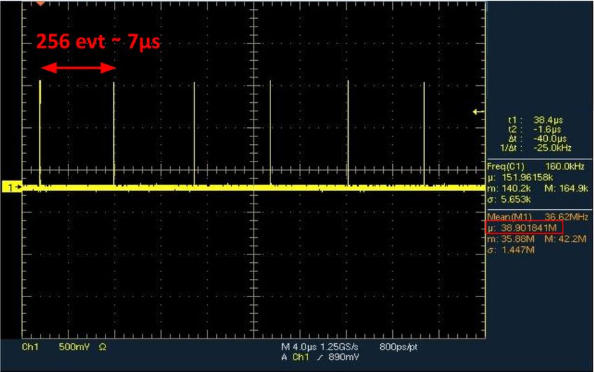
In order to run clustering as a real time process, the firmware has to sustain a 30 MHz
event processing rate, to sustain the LHC average bunch crossing rate. The system runs
comfortably without errors at a clock frequency of 350 MHz (out of a 650 MHz nominal
maximum for our chip model), providing a measured event rate of 38.9 MHz, as shown in
Fig. 8, amply sufficient to sustain the target rate of 30 MHz readout.
Figure 8. Oscilloscope screen shot showing the throughput test result. The FPGA board outputs a
signal every 256 events processed.
The firmware, completed with all necessary ancillary logic, has been integrated in the VELO
readout firmware as a self-contained block at the end of the processing chain; its output is
transmitted out of the readout card via PCIe interface.
A total of 52 Intel® Arria® 10 boards are needed to reconstruct the entire VELO, one
board for each module. Even if clustering data from a single VELO module does not require
all the FPGA resources available in an Intel® Arria® 10 chip, other operations need to be per-
formed beforehand. Those involve timing-alignment of SuperPixels and SuperPixel flagging
tasks [12] that add up to the total amount of resources needed. The resources needed for the
entire firmware, from receiving SuperPixels from the detector to cluster reconstruction, are
within the FPGA limits so no extra hardware is needed.
6 Throughput and bandwidth gains
VELO tracking, including cluster reconstruction, is the most time consuming task of the first
stage of the high level trigger (HLT1). It takes about 48% of the HLT1 processing time [13].
Running the HLT1 reconstruction on CPUs with and without the FPGA clustering algorithm
shows a gain in the event rate throughput of about 8%. LHCb has recently decided to run
the full HLT1 reconstruction on a GPU-based architecture starting from the imminent LHC
Run 3 [14]. The GPU-based HLT1 throughput increases by a factor of about 4% offloading
VELO clustering to FPGAs. Furthermore, running clustering at early DAQ stages reduces
the VELO detector bandwidth [15]. To quantify the reduction, the average number of SPs per
event is compared to the corresponding number of reconstructed clusters, leading to a data
size reduction of around 15%.
7EPJ Web of Conferences 251, 04016 (2021) https://doi.org/10.1051/epjconf/202125104016
CHEP 2021
7 Summary and outlook
We developed a FPGA-based 2D clustering algorithm for the LHCb silicon pixel detector,
capable of processing minimum-bias events at 38.9 MHz. The high processing rate, together
with the low amount of FPGA resources required, allows to run the algorithm in real time
during the detector readout. The clustering algorithm has been developed to exploit the full
flexibility and parallelization potential of FPGAs. The integration within the VELO read-
out firmware has been carried out, allowing significant throughput and bandwidth gains, thus
representing a promising alternative solution to more common CPU-based algorithms, with-
out extra costs. The algorithm physics performance is nearly indistinguishable from CPU
clustering and the feasibility of firmware installation in the readout boards has been carefully
studied. FPGA clustering is ready to be commissioned for use in physics data taking during
Run 3.
References
[1] LHCb Collaboration, JINST 3, S08005 (2008)
[2] LHCb Collaboration, Int. J. Mod. Phys. A 30, 1530022. 73 p (2014)
[3] LHCb Collaboration, Tech. Rep. CERN-LHCC-2011-001, CERN, Geneva (2011)
[4] F. Lazzari et al., J. Phys.: Conf. Ser. 1525, 012044 (2020)
[5] L. Giambastiani, A 2D FPGA-based clustering algorithm for the LHCb silicon pixel de-
tector running at 30 MHz, Master’s thesis, Università di Pisa, CERN-THESIS-2020-086
(2020)
[6] R. Cenci et al., PoS 313, 136 (2018)
[7] LHCb Collaboration, Tech. Rep. CERN-LHCC-2013-021, CERN, Geneva (2013)
[8] LHCb Collaboration, Tech. Rep. CERN-LHCC-2014-001, CERN, Geneva (2014)
[9] G. Bassi et al., FPGA implemention of a fast 2D clustering algorithm (VHDL language),
INFN Open Access Repository (2019)
[10] Dini Group® , https://www.synopsys.com/verification/prototyping/dini-products.html
(2021), Board model: DNS5GX_F2, Accessed: 2021-06-28
[11] Intel® Arria® 10 FPGAs, https://www.intel.com/content/www/us/en/products/
programmable/fpga/arria-10.html (2021), Accessed: 2021-06-28
[12] K. Hennessy et al., Readout firmware of the Vertex Locator for LHCb Run 3 and beyond,
Talk at 22nd Virtual IEEE Real Time Conference (2020)
[13] LHCb Collaboration, Tech. Rep. LHCB-FIGURE-2020-007, CERN, Geneva (2020)
[14] LHCb Collaboration, Tech. Rep. CERN-LHCC-2020-006, CERN, Geneva (2020)
[15] LHCb Collaboration, Tech. Rep. CERN-LHCC-2014-016, CERN, Geneva (2014)
8You can also read