3D printing path planning algorithm for thin walled and complex devices

Page created by Nancy Moreno
 
CONTINUE READING
3D printing path planning algorithm for thin walled and complex devices
Science and Engineering of Composite Materials 2021; 28: 327–334

Research Article

Min Yang*, Menggang Lai and Shengjun Liu

3D printing path planning algorithm for thin
walled and complex devices
https://doi.org/10.1515/secm-2021-0032                                  industry, 3D printing technology is widely used in medi-
received February 01, 2021; accepted June 03, 2021                      cal devices, aerospace, automobile manufacturing, and
Abstract: With the popularity of stereo printing technology,            other fields because of its low-cost production mode,
3D printers are widely used in industry, manufacturing,                 short cycle development time, and convenient and com-
medicine, and other industries to quickly manufacture                   plex process, and even known as the subversive tech-
small devices. Before 3D printing, it is necessary to plan              nology to promote the “third industrial revolution.” As
the printing path. Unreasonable printing path will not                  shown in Figure 1, common 3D printing technologies
only increase the time consumption of printing products,                mainly include stereolithography, fused deposition (FDM),
but also cause printing failure due to the accumulation of              selective laser sintering, and laser near net forming. No
stress and deformation in the printing process. In order to             matter what technology is selected, it is necessary to plan
overcome the superimposed stress and deformation in                     a reasonable printing path before printing, to make the 3D
the process of printing thin-walled complex devices,                    printing process fast and accurate and to improve the
this article introduces the idea of balanced stress based               printing efficiency and quality.
on the basic damage of the path planning based on the                        To plan a reasonable printing path, researchers have
potential field method. In the printing process, the ring                conducted extensive research on 3D printing path plan-
path, island path and cross path are added to overcome                  ning to improve printing efficiency and molding quality.
the stress deformation phenomenon and improve the                       The planning methods of reciprocating linear scanning
printing quality. Finally, the 3D printer is used to manu-              [1,2], which is a traditional way of 3D printing. Its tech-
facture thin-walled complex devices, and the feasibility                nology is relatively mature and has the characteristics of
of the balanced potential field method is verified by phy-                fast speed and simple algorithm. However, planning in
sical comparison.                                                       one direction will not only cause a lot of empty paths, but
                                                                        also lead to serious stress bending. In order to reduce
Keywords: 3D printing, path planning, potential field
                                                                        the time-consuming of empty paths in printing and to
method, balanced stress
                                                                        improve the printing efficiency, Rui-Shi et al. [3] applied
                                                                        “Z” planning algorithm to print devices. To some extent,
                                                                        it can reduce the warpage of printing, but it cannot solve
1 Introduction                                                          the problem of excessive burr at the inflection point. Lit-
                                                                        erature [4–6] proposes two simple algorithms and plans
3D printing technology, also known as a layered rapid                   the offset contour according to the model contour. In the
prototyping technology, is a kind of technology based                   process of printing, the path is planned step by step and
on the digital model file, which uses nylon glass fiber,                  layer by layer according to the object contour from out-
gypsum material, aluminum material, and other powder                    side to inside and from bottom to top. Although the
metal or plastic and other adhesive materials to manu-                  printing time and the edge burr are reduced, it is only
facture devices of arbitrary shape by slicing and accumu-               suitable for regular shapes with smooth boundary and
lating. Compared with the traditional manufacturing                     simple structure. In the process of step-by-step printing
                                                                        inward, “fracture” phenomenon is more serious [7]. The
                                                                        above methods consider devices to be printed as a whole,
                                                                      which are not suitable for special devices with “island.”
* Corresponding author: Min Yang, Structure Smart Construction
                                                                        Xiao-ya and Zheng et al. [8–10] divided the “isolated
R&D Center, CCCC First Highway Consultants Co., Ltd, Xi’an, 710065,
China, e-mail: yangmincccc@sina.com
                                                                        island” in the object into sections by the method of
Menggang Lai, Shengjun Liu: Structure Smart Construction R&D            type slicing to improve the printing quality. In addition,
Center, CCCC First Highway Consultants Co., Ltd, Xi’an, 710065, China   intelligent algorithms such as genetic algorithm, ant

   Open Access. © 2021 Min Yang et al., published by De Gruyter.         This work is licensed under the Creative Commons Attribution 4.0
International License.
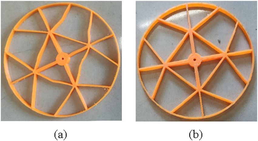
3D printing path planning algorithm for thin walled and complex devices
328         Min Yang et al.

                                                                                                                     3D prinng technology

                                                                                                                                                                                                                                                                                          Technology
                                Extrusion                                                 Line                            Granulaon                                         Laminated                                                            Beam
                                                                                                                                                                                                                                                 forming                                 classificaon
                                 forming                                                forming                            forming                                            forming

                                        Electron beam free forming

                                                                                                                                                                                                          Layered solid manufacture
                                                                                                                                                                             Selecve laser sintering
                                                                                              Electron beam melng

                                                                                                                                                                                                                                                              Digital light processing
                                                                                                                          Selecve laser melng

                                                                                                                                                  Selecve hot sintering
                                                                     Metal laser sintering
                     Melt straficaon

                                                                                                                                                                                                                                      Stereolithography
                                                                                                                                                                                                                                                                                         Technology
                                                                                                                                                                                                                                                                                         applicaon

Figure 1: Common 3D printing technology.

colony algorithm, hash algorithm and Hilbert curve                                                                                                                         path is constantly changed, so that the algorithm can
method [11–14] are also applied to 3D printing to find                                                                                                                      completely traverse the global environment. The prin-
new and efficient planning methods.                                                                                                                                          ciple is that in the process of path planning, the target
    Although these algorithms improve the 3D printing                                                                                                                      position is set to attract the next trend of the path, and
performance to a certain extent, they are not suitable for                                                                                                                 the repulsion position is set to prevent the path. In the
the special case of thin-walled devices. In order to improve                                                                                                               global process, the potential function Usum is the super-
the efficiency of 3D printing, this article proposes a path                                                                                                                  position of gravitational function Uatt and repulsive func-
planning method based on balanced potential field (BPF)                                                                                                                     tion Urep .
algorithm. The reasonable printing path is quickly planned                                                                                                                                                                                                Usum = Uatt + Urep                            (1)
by using the balanced field method. Based on this the stress
deformation is abstracted as a potential field function, and                                                                                                                    The gravity function Uatt is defined as a monotonic
the stress is reduced by the method of BPF. Force deforma-                                                                                                                 function that grows with the distance function d(n , ngoal)
tion can not only effectively print thin-walled complex                                                                                                                     between the current position node n and the target node ngoal
devices, but also greatly reduce the warping of edge area
                                                                                                                                                                                                                    1 ξd 2 ,                        ⁎
                                                                                                                                                                                                                                                d ≤ dgoal
in printing process, and improve the success rate and                                                                                                                                                              2
                                                                                                                                                                                                         Uatt(n) =               1
                                                                                                                                                                                                                                                                                                        (2)
quality of printing.                                                                                                                                                                                                ξdgoal
                                                                                                                                                                                                                        ⁎             ⁎
                                                                                                                                                                                                                              d − 2 (dgoal           ⁎
                                                                                                                                                                                                                                           )2 , d > dgoal
                                                                                                                                                                                                                   
                                                                                                                                                                           where d = d(n , ngoal), ξ is the gravitational coefficient and
                                                                                                                                                                            ⁎
                                                                                                                                                                           dgoal is the gravitational threshold function.
                                                                                                                                                                                The gravitational potential field function Diff(Uatt) is:
2 3D printing path planning based
                                                                                                                                                                                                                         ξ (n − ngoal),             ⁎
                                                                                                                                                                                                                                                d ≤ dgoal
  on BPF method                                                                                                                                                                                                         
                                                                                                                                                                                                        Diff(Uatt(n)) =  ⁎ n − ngoal                ⁎                                                  (3)
                                                                                                                                                                                                                         ξdgoal d(n , ngoal) , d > dgoal
                                                                                                                                                                                                                        
2.1 Potential field method
                                                                                                                                                                               In path planning, the unexpected area is represented
                                                                                                                                                                           by repulsion function. Therefore, the repulsion function
Extensive research on potential field methods has proved
                                                                                                                                                                           of calculation point Uatt(n) should be inversely correlated
the effectiveness in path planning, but those research
                                                                                                                                                                           with the distance function d(n , nrep) between the current
mainly focuses on robots and unmanned aerial vehi-
                                                                                                                                                                           position node n and the calculated repulsion node nrep
cles [15,16].
    The main idea of path planning using the potential                                                                                                                                                                                    1  1    1 
field (PF) is to find the global potential field function. In                                                                                                                                                                                 η  − ⁎  d ≤ drep
                                                                                                                                                                                                                                                               ⁎
                                                                                                                                                                                                                                Urep(n) =  2  d  drep                                                (4)
the process of path planning, the path that has been                                                                                                                                                                                       
                                                                                                                                                                                                                                           0                  ⁎
                                                                                                                                                                                                                                                          d > drep
traversed and the potential field target in the unknown                                                                                                                                                                                     
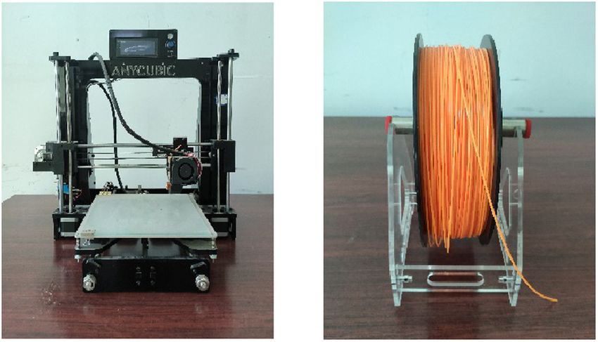
3D printing path planning algorithm for thin walled and complex devices
3D printing path planning algorithm                     329

     The repulsion potential field function Diff(Urep) is as
follows:

                  1      1 1
                 η  ⁎ −  2 (drep
                                   ⁎              ⁎
                                       − d), d ≤ drep
Diff(Urep(n)) =   drep   dd                           (5)                 3D prinng path direcon   Stress and deformaon direcon
                 
                  0,                             ⁎
                                             d > drep
                 
                                                         ⁎
where d = d(n , nrep), η is the repulsion coefficient and drep
is the repulsion threshold function.
     By superposing the repulsion functions of all calcu-
lation points in the repulsion region, the repulsion func-
tion Urep can be formed as:
                            N
                      Urep = ∑ Urep(n)                   (6)
                                                               Figure 2: Stress deformation diagram.
                            n=1

    In path planning, based on completing the current
path point, the gradient direction of the next step is the     thin-walled edge. As shown in Figure 2, a plane in the
superposition direction of the gravitational gradient field     printing process is extracted, in which the black arrow
and the repulsive gradient field:                               represents the print path and the red arrow indicates the
         Diff(U (n)) = Diff(Uatt(n)) + Diff(Urep(n))     (7)   stress direction. At the edge of the device, due to the
                                                               stress warping, the device is easy to deform, resulting
     If the printed path points and blank areas are set as     in printing failure. Moreover, because only the potential
repulsive points, and the unprinted path points are gravity    field method is used to print step by step and line by line,
points, the global path can be traversed by using the          the warping is more serious, even leading to the printing
potential field method. Although the ergodic potential          failure of the whole device.
field method has great advantages in fast path planning,             The main idea of the BPF method is to balance the
the application to 3D path planning is not much. Yu-jie [17]   sudden change of stress direction at the edge of the
introduced the potential field method into the path plan-       device and the stress superposition in the process of
ning, and finally determined the optimal traversal path         the device plane printing step by step. To eliminate this
through the fast traversal method. Xiao-lei et al. [18] com-   adverse effect, it is necessary to change the path direction
bined the grid complete traversal with artificial potential     in real-time according to the stress change trend in the
field method, so that the planned path has better perfor-       printing process, as shown in Figure 3, to plan the cir-
mance in practicability, rationality and real-time.            cular path, cross path, and island path, so as to reduce
     The potential field method has great potential in the      the stress deformation effect.
path planning of 3D printing, but the disadvantages are
also obvious [19]. In the printing process, only how to
traverse the path quickly is considered, but the stress        2.2.2 Algorithm derivation
mutation in the printing process is ignored, for example,
the edge is easy to warp and the joint is easy to deform. It   Before 3D printing, assuming that the global path of the
is necessary to improve the PF method to improve the           printed device is a two-dimensional point set G(X , Y ), the
printing quality and success rate.                             current printing location is pnow = (xnow , ynow), the next step
                                                               is to predict the printing path point as pnext = (xnext , ynext),
                                                               the optimal trend point as popt = (xopt , yopt), the available
2.2 Balanced potential field method
                                                               gravitational function Uatt(pnext ) and repulsive function
                                                               Urep(pnext ) are as follows:
2.2.1 Basic thought
                                                                                     1 2                          ⁎
The traditional potential field method only considers the                              2 ξd ,                d ≤ dnext
                                                                      Uatt(pnext ) =                                                    (8)
optimization of the printing path but ignores the stress of                            ξdnext
                                                                                           ⁎      1 ⁎ 2            ⁎
                                                                                              d − (dnext ) , d > dnext
special printing positions such as inflection point and                                           2
330          Min Yang et al.

                                                                               B(X , Y ) = ψ ⋅ G(X , Y ), B(X , Y ) ∈ G(X , Y )        (11)

                                                                            For any printing path L(X , Y ) ∈ B(X , Y ), take contin-
                                                                       uous two points p1 = (x1, y1) ∈ L and p2 = (x2 , y2) ∈ L given
                                                                       in the printing process on path L, and define the deforma-
                                                                                   →
                                                                       tion stress Fp2 → p1 of p2 to p1 as:
                                (a)                                                        →               →      1
                                                                                           Fp2 → p1 = γ ⋅ p2 p1 × →                    (12)
                                                                                                                  L
                                                                       where γ is the deformation force calculation coefficient, ×
                                                                       is the cross multiplication symbol, the deformation force
                                                                       →                                                      →
                                                                       Fp2 → p1 obtained is the normal direction formed by p2 p1
                                                                              →
                                                                       and L , as shown in Figure 4.
                                                                              It can be concluded that the superimposed deforma-
                                                                                     →
                                (b)                                    tion force F →  L on the path L is the superposition effect
                                                                       force of the sum of all continuous two points pi =
                                                                       (xi , yi) ∈ L and pj = (xj , yj) ∈ L:

                                                                                           →→           →    1
                                                                                           F L = ξ ∑ pi pj × →                       (13)
                                                                                                   i, j      L
                                                                               →
                                                                            If F →
                                                                                 L is greater than the threshold value, it may cause
                                                                       stress deformation of the device, even lead to the failure
                                (c)                                    of printing in B(X , Y ). When the superposition effect force
                                                                       →→
                                                                       F L is close to the deformation threshold force, the path
Figure 3: Planning path to overcome stress deformation. (a) Circular   →
path. (b) Cross path. (c) Island path.                                 L should be truncated to eliminate the superposition
                                                                       effect of stress, that is to balance the stress potential field.
                         1  1     1          ⁎
                                                                       According to the different situations encountered in printing,
                          η      − ⁎ , d ≤ dnext
          Urep(pnext ) =  2  d  dnext                       (9)    ring path, cross path, and island path are planned respec-
                                               ⁎                      tively to balance the stress potential field.
                          0,              d > dnext
                                                                       (1) Printing path based on balanced stress potential field
                                                             ⁎                   For a printing path L(X , Y ), if the current super-
where          d=     (xnow − x )2 + ( ynow − y )2 ,        dnext =
                                                                                                   →
                                                                            imposed effect force F →  L is greater than the set stress
 (xnow − xnext)2 + ( ynow − ynext)2 and (x , y ), (xnow , ynow),
                                                                            threshold, the cross path needs to balance the current
(xnext , ynext) ∈ G(X , Y ).                                                stress and reduce stress deformation. The optimal
     The resultant force of potential field function U (pnext )              point of the next printing path popt is as follows:
is obtained as follows:
                                                                                                 p ,                →         L
                   1                                                                             next             ∣F →
                                                                                                                       L ∣ < Fthresh
                            1 1        1           ⁎                                  popt    =                   →                 (14)
                    ξd 2 + η  − ⁎ , d ≤ dnext                                                  p balance ,      ∣F →       L
                   2       2 d       dnext                                                                         L ∣ ≥ Fthresh
      U (pnext ) =                                       (10)
                    ξd ⁎ d − 1 (d ⁎ )2 ,      d > d ⁎
                    next         next               next
                             2
                                                                                                               ur
    If there is U (pnext ) ≥ U (p) for any p = (x , y ) ∈ G(X , Y ),
                                                                                                               F p2o p1
then the optimal trend point of the next printing path is
popt = pnext . Although the printing path can be drawn
according to the potential field law, the problem of stress                                     ur
                                                                                               L                          ur
and deformation is not eliminated. Therefore, the region                                              uuuuur
                                                                                                      p2 p1               L
of balanced potential field B(X , Y ) is introduced to bal-
ance the problem of global uneven stress G(X , Y ).
    Define B(X , Y ) as a partial region of G(X , Y ):                  Figure 4: Force deformation diagram.
3D printing path planning algorithm         331

    where p balance is the direction point perpendicular to
    pnext . When the algorithm feels that the path may
    produce stress deformation, it balances the stress
    deformation effect by changing the printing path
    direction to a normal direction perpendicular to the
    original direction.
(2) Printing area based on balanced stress potential field                 Figure 5: Connecting path of balanced force potential field at the
         For a partial area of the device B(X , Y ) ∈ G(X , Y ),          edge of thin wall.
    the path of the printing area is L1 , L2 , L3 ,… Lj , it can be
    considered that the region is equal to the superposi-
    tion of multiple paths:                                                   In other words, the path C of the edge can be
                      B(X , Y ) ≈ {L1 , L2 , L3,… Lj} (15)                divided into two cases according to the relationship
                                                                                   →
                                                    →                     between FC and the maximum deformation stress
        Then the stress superposition of the region FB is                            C
                                                                          threshold Fthresh :
    calculated as the superposition stress of each path:
                                                                                   {p , p , p , … p },                 →      C
                   → →→ →→ →→                  →
                   FB = F L1 + F L2 + F L3 + ⋯ F →                                  1 2 3             m               ∣FC∣ < Fthresh
                                                 Lk                              C=                                    →               (18)
                          →→                                                       {p1 , p2 , p3 , … pm , L p1 pm},           C
                                                                                                                       ∣FC∣ ≥ Fthresh
                      = ∑F Lk                                                      
                           k                                       (16)
                                                                              The BPF method can be used in 3D printing for thin-
                                   →   1                                walled complex devices based on three situations. By
                       == ξ ∑∑ pi pj × → 
                                   
                            k i, j 
                                                                         calculating the relative situation of superimposed stress
                                        Lk 
                                                          →               and stress threshold, the superimposed stress effect can
         When the superimposed stress of the region FB is                 be cut off, and the printing quality and success rate can
    greater than the maximum deformation stress threshold                 be improved.
      B
    Fthresh , the stress and deformation of a small part of the
    region may occur. Therefore, when the stress super-
    position approaches the maximum deformation stress
    threshold, the island path Θ = {l1, l2 , l3, … ln} is re-
    planned in the region to balance the device deformation               3 Algorithm flow of 3D printing
    caused by regional stress superposition. The printing
    area B(X , Y ) is:
                                                                            path planning based on balanced
                {L , L , L , … L },               →       B
                                                                            potential field method
                 1 2 3               j           ∣FB∣ < Fthresh
    B(X , Y ) ≈                                   →               (17)
                 B − Θ , {l1, l2 , l3, … ln}},            B
                                                  ∣FB∣ ≥ Fthresh          Figure 6 is the algorithm flow chart of 3D printing path
                
                                                                          planning based on BPF method.
(3) Printing thin-walled edge based on balanced stress                         After the algorithm starts to run, the parameters are
    potential field                                                        initialized and their initial values are set, then the current
        For thin-walled complex devices, the stress bal-                  print node is obtained. Based on the current print node,
                                                          →
    ance method of edge is similar to print path. If FC                   the next step print node is planned. According to the
    is greater than the maximum deformation stress                        gravity function and repulsion function of the global
                 C                                                        node, the next optimal print node is obtained until all
    threshold Fthresh  of thin-walled edge, circular path is
    needed to balance the stress. It should be noted that                 nodes of the device are traversed to generate the planned
    the path C = {p1 , p2 , p3 ,… pm } of thin-walled edge                print path. At this time, the BPF method is introduced
    needs to contain at least one connecting path to con-                 to determine whether there are paths and areas that
    struct a circular path. As shown in Figure 5, when cal-               may produce stress deformation in the generated path.
    culating the stress of the thin-walled edge (blue curve),             According to different situations, the balanced printing
    there must be one connecting path at least (red line                  path, balanced printing area and balanced thin-walled
    segment) to make C end to end.                                        edge are used to balance all the stress within the
332         Min Yang et al.

                                           Start
                                                                                                               Balanced potenal
                                                                                                                  field method
                                        Inializaon
                                         K ǃ[ ǃJ
                                                                                                                                  ur
                                                                    Balanced         ­^ p1 , p2 , p3 ,L pm `                  ,           C
                                                                                                                                  F C  Fthresh
                                                                                     °
                                                                    printing      C= ®                                            ur
                                     Current print                    path              ^
                                                                                     °̄ p1 , p2 , p3 ,L pm , Lp1 pm   `   ,               C
                                                                                                                                  F C t Fthresh
                                       node n

                         Gravitaonal               Repulsion                                                                       ur
                                                                    Balanced               ­^L1 , L2 , L3 ,L L j `          ,               B
                                                                                                                                    F B  Fthresh
                           funcon                   funcon                               °
                                                                    printing      B X ,Y | ®                                       ur
                          U att pnext                 U rep pnext                          °̄^B  4ˈ^l1 , l2 , l3 ,L ln `` ,
                                                                                                                                            B
                                                                                                                                   F B t Fthresh
                                                                      area

                                     Next opmal
                                     node popt                                                                   ur ur
                                                                    Balanced             ­ pnext ,                        L
                                                                                                                 F L  Fthresh
                                                                                         °
                                                                     printing
                                                                                  popt = ®                       ur ur
                                                                    Thin wall                                            L
                                No        Planning                                       °̄ pbalance ,           F L t Fthresh
                                                                      edge
                                         completed?

                                              Yes

                                                                                     The stress is balanced                             No
                                                                                  within the threshold range?

                                                                                                        Yes

                                                                                                   End

Figure 6: Algorithm flow of 3D printing path planning based on balanced potential field method.

threshold range and to improve the printing efficiency                            balanced potential field method is in G-code format
and success rate.                                                               and the point set part of the path planning is replaced,
                                                                                the absolute control of the nozzle can be carried out
                                                                                according to the designed path.

4 Comparative experiment and
  analysis

4.1 Configuration of 3D printing environment

Before comparing 3D printing, we need to configure the
experimental environment. The 3D printer used and its
printing consumables are shown in Figure 7. It can carry
out secondary development for the self-developed plan-
ning program and printing path.
    It adopts the printing principle of FDM and Cura sli-
cing software to output designed model under the three-
dimensional software ring as G-code for common path
planning and 3D printing. If the path planned by the                            Figure 7: Arm-based 3D printer and consumables.
3D printing path planning algorithm          333

4.2 Experimental verification

For practical comparison, the general potential field (GPF)
method and the balanced potential field method are used
respectively for the 3D printing of thin-walled complex
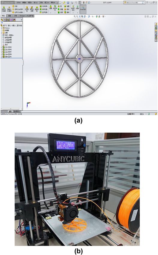
devices. For example, Figure 8(a) is the model of thin-walled
complex devices planned by computer, and Figure 8(b)
shows the equipment and devices.
    The devices printed by GPF and BPF are shown in
Figure 9(a) and (b), respectively. The device printed by
the GPF method has serious deformation. When printing
                                                                       Figure 9: 3D printing thin-walled complex device. (a) GPF method
thin-walled connections, the GPF method always prints
                                                                       and (b) BPF method.
in the same direction, it is easy to produce stress defor-
mation, which makes the printed device partially deformed
and difficult to meet the quality of high-precision printing.            the characteristics of the virtual model and overcome the
But the device printed based on BPF method can maintain                stress effect.
                                                                            To make a more intuitive comparison between BPF
                                                                       and GPF, both algorithms for 3D printing are tested 10
                                                                       times. From the formal operation of the 3D printing
                                                                       machine to the end of the device printing, the printing
                                                                       time and the quality of the printed device are recorded,
                                                                       respectively, and the results are shown in Figure 10. (The
                                                                       quality of the device is defined as the number of lines
                                                                       without stress deformation. The maximum number of
                                                                       line segments of the device is 32, so the best-printed
                                                                       quality of the device is 32.)
                                                                            The printing time of the GPF method is less than BPF,
                                                                       but the printing effect is not satisfactory. The GPF method
                                                                       can only print a small number of good line segments,
                                                                       moreover, it cannot control the printing quality, with
                                                                       large variance and many defective products. While the
                                                                       BPF method sacrifices a small part of printing time to
                                                                       exchange for printing quality, which not only improves
                                                                       the printing quality but also ensures that the stress

                                                                       Print me                                                      Print quality

                                                                                1          2    3     4    5          6   7   8   9   10
                                                                             Print me                         B PF                   G PF
Figure 8: 3D printing model and devices in printing. (a) Thin-walled       Print quality                       BPF                    GPF
and complex device model. (b) Equipment and devices in printing
process.                                                               Figure 10: Result of two path planning algorithms.
334           Min Yang et al.

deformation is reduced as much as possible in each 3D                    [5]    Wen-jun X. Variable distance offset filling algorithm for
printing. The success rate of thin-walled complex devices                       Centroid contraction[D]. Wuhan: Huazhong University of
is greatly improved.                                                            Science and Technology; 2007.
                                                                         [6]    Zhong-wei L, Chang-biao H, Ze-hao W. Algorithm on genera-
                                                                                tion of spiral filling path for planar con-tour. Comp Eng Appl.
                                                                                2015;51(18):180–5.
                                                                         [7]    Serra T, Ortiz-Hernandez M, Engel E, Planell JA, Navarro M.
5 Conclusion                                                                    Relevance of PEG in PLA-based blends for tissue engineering
                                                                                3D-printed scaffolds. Mater Sci Eng. 2014;38(1):55–62.
                                                                         [8]    Xiao-ya Z, Fa-lai C. 3D printing path planning of fractal models.
This article first briefly introduces the path planning pro-
                                                                                J Comput Des Comput Graph. 2018;30(06):1123–35.
cess of GPF, summarizes its advantages and disadvan-                     [9]    Zheng Y, Pan M, Chen F. Boundary correspondence of planar
tages. Then GPF is improved to BPF, to balance the stress                       domains for isogeometric analysis based on optimal mass
and deformation, which improves the strength of each                            transport. Comput Aided Des. 2019;114:28–36.
print segment. Finally, actual devices are printed out by                [10]   Yan-li T, Yong-qiang Z. Research on 3D image optimization and
                                                                                segmentation of 3D print geometry. Comput Simul.
a 3D printer. Comparative experiments and analyses have
                                                                                2018;35(8):165–9.
proved the effectiveness of BPF method.
                                                                         [11]   Xing-guo H, Xiao-hui S, Ming Y, Hai-jun C, Guo-fu Yin. Path
    Although the possible extension of this work has                            optimization algorithm of 3D printing based on fused deposi-
great prospects, still there are several issues in need of                      tion modeling. Trans Chin Soc Agric Machinery.
further study.                                                                  2018;49(3):393–401.
(a) In this article, a thin-walled device is printed, but the            [12]   Yan-yan Z. Research on 3D printing path planning technology
                                                                                based on FDM Technology. Changchun: Changchun University
    extension of BPF method to big prototypes needs
                                                                                of Technology; 2016.
    more study.                                                          [13]   Li-gang L, Wen-peng X, Wei-ming W, Zhou-wang Y, Xiu-liu P.
(b) Research on putting this work from theory to struc-                         Survey on geometric computing in 3D printing. Chin J Comp.
    tural study needs further study.                                            2015;6:1243–67.
                                                                         [14]   Feng-ying C, Xiao-wei L. Research on 3D printing path plan-
Conflict of interest: Authors state no conflict of interest.                      ning. J Qingdao Univ Sci Technol (Nat Sci Ed).
                                                                                2020;41(2):101–5.
                                                                         [15]   Liu S, Zhang Q, Zhou D. Obstacle avoidance path planning of
                                                                                space manipulator based on improved artificial potential field
                                                                                method. J Inst Eng (India): Ser C. 2014;95(1):31–9.
                                                                         [16]   Ren J, McIsaac KA, Patel RV. Modified Newton’s method
References                                                                      applied to potential field-based navigation for nonholonomic
                                                                                robots in dynamic environments. Robotica.
[1]   Rajan VT, Srinivasan V, Tarabanis KA. The optimal zigzag                  2008;26(1):285–94.
      direction for filling a two-dimensional region. Rapid Prototyp J.   [17]   Yu-jie C. Research on path planning method of RoboCup
      2001;7(5):231–41.                                                         medium group soccer robot [D]. Changsha, Hunan, China:
[2]   Asiabanpour B, Khoshnevis B. Machine path generation for the              Changsha University of Technology; 2015.
      SIS process. Robot Comput-Integ Manuf. 2004;20(3):167–75.          [18]   Xiao-lei L, Lin J, Zu-fei J, Chen G. Mobile robot path planning
[3]   Rui-shi T, Ming-yao L, Fan Z, Yue-gang T. Continuous path                 based on environment modeling of grid method in
      planning algorithm for carbon fiber composite material 3D                  unstructured environment. Mach Tool Hydraul.
      printing. Mach Des Manuf. 2019;6:1–4.                                     2016;44(17):1–7.
[4]   Chang-biao H, Kai-yong J, Jun-yi L. Research on algorithm for      [19]   Jia YL. Research on 3D printing path planning algorithms
      contour lines offset and interference elimination. Mech Electr             based on reinforcement learning. Dalian: Dalian University of
      Eng Technol. 2007;36(10):75–7.                                            Technology; 2019.
You can also read