3D printing for mathematical visualisation
←
→
Page content transcription
If your browser does not render page correctly, please read the page content below
3D printing for mathematical visualisation∗
                                         Henry Segerman

1        Introduction
3D printing is quickly becoming a very affordable option for producing physical
objects. The term “3D printing” covers a number of closely related technologies,
all of which produce a 3-dimensional physical object from a computer model by
building it up in successive layers. These technologies were developed primarily
for use in rapid prototyping for industrial design; they allow a designer to convert
a computer model of a prototype into a physical object quickly in comparison to
most previously available technologies. In addition, there are a number of other
advantages that make 3D printing attractive for making mathematical models.

    1. There is a huge amount of freedom in the geometry that may be produced.
       With “subtractive” manufacturing techniques, in which material must be re-
       moved from an initial solid (e.g. lathing, drilling or carving), objects with
       intricate internal structure can be very difficult to produce. With 3D print-
       ing’s “additive” procedure, these problems are greatly mitigated.

    2. The resulting object very closely approximates the mathematical ideal of the
       model. The workflow is

                  Mathematical concept → computer model → 3D printed object

          The first arrow might involve construction “by hand” within a 3D computer-
          aided-design program, or the geometry might be constructed using a program
          (e.g. a Python script) written by the user. In either case, the geometry of
          the computer model can be extremely faithful to the mathematical concept.
          The second arrow is dealt with by a 3D printer, and these are typically
          accurate to a fraction of a millimetre.

    3. 3D printing does not have large initial setup costs (in contrast to the process
       of casting from a mould for example, which must be produced first, often at
       large expense).

On the subject of affordability, there are now a number of web-based companies
that will 3D print your models for you, at very reasonable prices, so it is not nec-
essary to own or have access to a 3D printer to be able to get started. Having said
that, many colleges and universities have purchased 3D printers for use in archi-
tecture or design departments. The main advantage of having direct access to a
    ∗
        This is a preprint. The final publication is available at www.springerlink.com, at this page.

                                                   1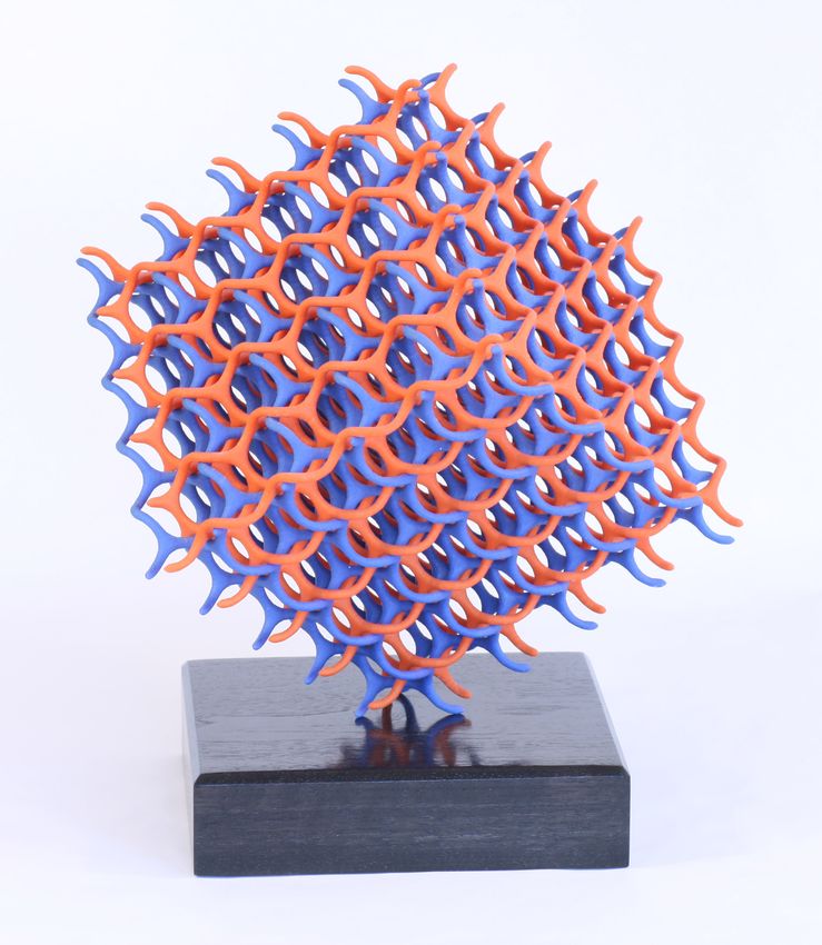
3D printer is turn-around time: depending on the size of the object, the printing
itself generally takes several hours. However, with a web based company, it might
take a week or two to go from uploading a design to their website to having the
3D printed object in one’s hands.
This article is in two parts. The first shows some recent 3D printed work by a
number of mathematicians and mathematical artists, which will hopefully inspire
the reader to try out the second part, which is a tutorial on producing a 3D design
of a parametrically defined surface. In terms of software, the tutorial only requires
access to Mathematica [15]. To go along with this article, I have also written de-
tailed instructions on using one of the 3D printing services to fabricate your design,
and some notes on going further in producing objects using 3D printing. These
notes are available at http://www.segerman.org/3d_printing_notes.html.

2     Examples of 3D printed visualisations
George Hart has written previously in the Mathematical Intelligencer on 3D printed
mathematical visualisations [9], covering models of the Sierpinski Tetrahedron and
the Menger Sponge, as well as various polyhedral designs and projections of 4-
dimensional polytopes. Figure 1 shows one of his more recent works, based on the
crystal structure (10,3)-a, described by the chemist A.F. Wells. See [8] for more
details. Bathsheba Grossman is an artist working mostly in 3D printed metal.
The two examples shown in Figure 2 illustrate a technique developed by her to
represent a surface with perforations. The sizes of the holes are related to the
curvature of the surface. See [7]. Carlo Séquin is a computer science professor,
and often teaches courses involving computer modelling and 3D printing. Two
of his recent works are shown in Figure 3, and many more can be found at [14].
Some 3D printers are able to print directly in colour, as in Figures 1b and 3b.
David Bachman (Figure 4) and Burkard Polster (Figure 5, also see [12]) are both
mathematicians whose 3D designs are available on shapeways.com, one of the
web-based 3D printing services. I have also included two designs by myself in
collaboration with Saul Schleimer in Figure 6. These objects are native to the
three-dimensional sphere, S 3 , and are mapped to R3 via stereographic projection
so they can be printed. See [13] for details. Note that the 3D printed objects
in Figures 1b and 6b(lower) consist of two parts that are intricately interlinked.
This kind of object would be extremely difficult to manufacture other than by 3D
printing.
    There are a number of other mathematical artists working with 3D printing.
See also work by Vladimir Bulatov [4], whose designs involve polyhedral sym-
metry or 3-dimensional hyperbolic geometry and “Nervous System” [11], who use
computer simulation of natural processes, for example reaction-diffusion.

3     Getting started in 3D printing
3.1   Software
There are many more-or-less fully featured 3D design programs. These range
from very expensive programs used in films and computer games (e.g. 3ds Max

                                          2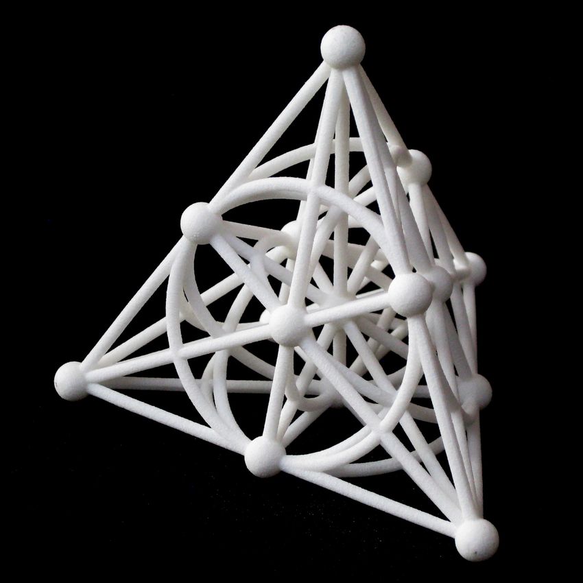
(a) A 4 × 4 × 4 block of the lattice structure.       (b) Two mirror image copies of the lattice
                                                       interlinked with each other.

      Figure 1: The crystal structure (10,3)-a, 3D print design by George Hart.

 (a) The gyroid, a triply periodic minimal             (b) A Seifert surface with boundary the Bor-
 surface discovered by Alan Schoen.                    romean rings.

                        Figure 2: Designs by Bathsheba Grossman.

[2], Maya [3]), through to free and open-source software (e.g. Blender [6], MeshLab
[5])1 . Many of the commercial programs have large educational discounts, although
even so they can be relatively expensive. Of the free software, Blender is very full
featured, but (at least at the moment) has a somewhat non-standard user interface
and steep learning curve. MeshLab has far fewer features, but is useful for viewing
and making small changes to mesh files (the data that is sent to a 3D printer).
Both Blender and MeshLab have versions for Windows, OS X and Linux. I mostly
  1
      Note that this is a very incomplete list.

                                                   3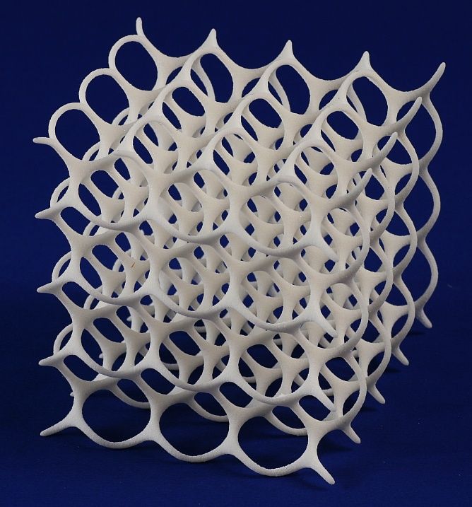
(a) “Hilbert Cube 3D”, a step in the con-            (b) “Symmetrical Half-way Point for Torus
 struction of a space filling curve.                  Eversion”.

                            Figure 3: Designs by Carlo Séquin.

 (a) A hyperbolic paraboloid, showing slices          (b) A hyperbolic paraboloid, showing level
 through the surface in the x and y directions.       curves.

                          Figure 4: Designs by David Bachman.

use a commercial program called Rhinoceros [1] (or just Rhino), which is available
for Windows, with an OS X version currently in open beta. As with many of these
software packages, Rhinoceros has a scripting language (including a version based
on Python), with which it is possible to generate geometry procedurally. It is
also easy to make “ruler and compass”-like constructions in 3D, and it can import
2-dimensional geometry from Adobe Illustrator. I also use MeshLab as a sanity
check for any mesh files I make before sending them to a printer.
Becoming familiar with one of these programs is a good idea going further, but we
can get quite far using Mathematica alone. Since readers of this article are quite

                                                  4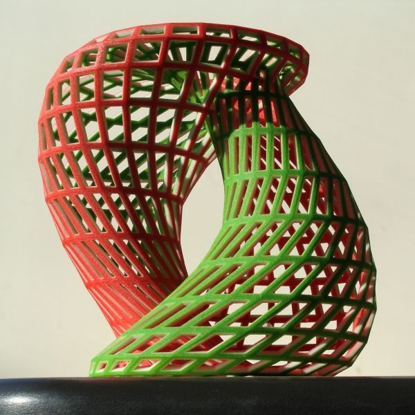
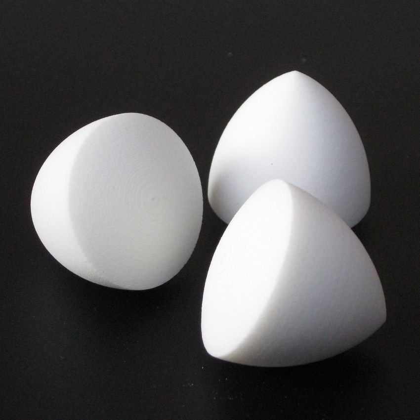
(a) A solid of constant width, made by ro-         (b) A representation of P G(3, 2), the small-
  tating a Reuleaux triangle around one of its       est finite projective space.
  symmetry axes.

                        Figure 5: Designs by Burkard Polster.

  (a) An unusual parameterisation of a punc-               (b) Dual Half 120- and 600-cells
  tured Möbius strip.

       Figure 6: Designs by the author in collaboration with Saul Schleimer.

likely to have access to Mathematica, we will generate an example visualisation
using it.

3.2    Example: generating a parametric surface using Mathemat-
       ica
Inspired by Bachman’s models in Figure 4, we will produce a grid-like represen-
tation of a parametrically defined surface, in this case a hyperbolic paraboloid.
The Mathematica code2 for this is in the next section. Models like this could be
very useful pedagogical tools in a multivariable calculus class for example. The
graphical output of the code is shown in Figure 7a.
   2
    I have tested the code in Mathematica 7 and 8, and it should hopefully run in some earlier
versions as well.

                                                 5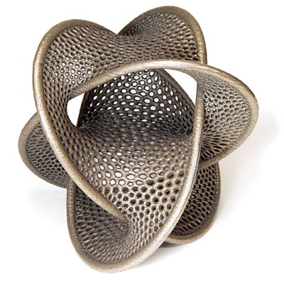
(a) Graphical output from Mathematica.             (b) The STL file as viewed in MeshLab.

               Figure 7: Generated model of a hyperbolic paraboloid.

    In addition to this graphical output, the code also exports the graphics data
as a mesh in the “STL” 3 file format. The file “MathematicaParametricSurface.stl”
should appear in your root directory when the code is run. In Figure 7b we see
this file as viewed in MeshLab. The STL file format is a standard format for
describing a mesh of triangles, and is one of the formats that 3D printers take as
input. The file essentially consists of a long list of triangles, each triangle given by
the coordinates in 3-dimensions of its three corners. A 3D printer takes this list of
triangles and interprets their union as a closed orientable embedded surface in R3 ,
from which it can determine which voxels (3-dimensional analogues of pixels) are
inside the surface (and so should be solid, filled with plastic or whatever material
the printer is using), and which are outside the surface (and so should be empty).
Some programs (for example MeshLab) allow you to export in an ASCII version
of STL (as opposed to the usual binary version), which results in a much larger file
size, but the file can also be read in any text editor, and the triangle coordinates
can be read manually4 .
    Before going into detail on how the code works (and so how to modify it!), a
few words are in order on the choice of representation of the surface. A surface
is 2-dimensional, but any real world representation of it must have some non-
zero thickness. The idea used here is to draw curves on the surface given by
keeping one of the two parameters constant. We “thicken up” these curves using
regular tubular neighbourhoods of them. Instead, we could have thickened up
the whole surface rather than just these curves, in effect filling in the rectangular
holes in the surface. There are a few reasons that I tend to avoid this. First,
this uses more material, and generally this means that the object will be more
expensive to produce. Second, the pattern can give a better visual sense of the
   3
    “STL” stands for “Standard Tessellation Language”.
   4
    If one were so inclined, one could write a program to output this STL format directly,
bypassing the need for any 3D software. In most cases however, this would involve the reinvention
of numerous wheels.

                                               6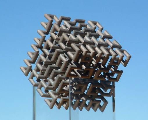
shape of the object than a blank, featureless surface does, and it also communicates
     mathematical content in terms of the parameterisation. Third, it can be useful to
     be able to see partially through the surface to other features behind it.

     3.3     Mathematica code
     Here is the code to generate the graphical output shown in Figure 7a, together
     with the STL file.
 1   f [ u_, v_ ] := {u , v , u^2 − v ^ 2 } ;
 2   scale = 40;
 3   radius = 0.75;
 4   numPoints = 2 4 ;
 5   gridSteps = 10;
 6   curvesU = Table [ s c a l e ∗ f [ u , i ] , { i , −1, 1 , 2/ g r i d S t e p s } ] ;
 7   curvesV = Table [ s c a l e ∗ f [ j , v ] , { j , −1, 1 , 2/ g r i d S t e p s } ] ;
 8   tubesU = ParametricPlot3D [ curvesU , {u , −1, 1 } , PlotStyle −> Tube [
            r a d i u s , PlotPoints −> numPoints ] , PlotRange −> All ] ;
 9   tubesV = ParametricPlot3D [ curvesV , {v , −1, 1 } , PlotStyle −> Tube [
            r a d i u s , PlotPoints −> numPoints ] , PlotRange −> All ] ;
10   c o r n e r s = Graphics3D [ Table [ Sphere [ s c a l e f [ i , j ] , r a d i u s ] , { i , −1, 1 ,
            2 } , { j , −1, 1 , 2 } ] , PlotPoints −> numPoints ] ;
11   output = Show [ tubesU , tubesV , c o r n e r s ]
12   Export [ " M a t h e m a t i c a P a r a m e t r i c S u r f a c e . s t l " , output ]

         • Line 1 gives the parametric function f : [−1, 1]2 → R3 that defines the
           parametric surface patch. This, of course, can be altered to give any desired
           parametric surface.

         • Line 2 defines a scaling factor, which the geometry is scaled up by in the final
           model. Our units will be in millimetres, and so the x-coordinate bounds of
           our model will be approximately −1 × 40 to 1 × 40, which is 80 millimetres,
           or 8 centimetres. Similarly for the y-coordinate bounds.

         • Line 3 gives the radius of the tubular neighbourhoods around the curves,
           again in millimetres. Depending on the choice of material and printer, a
           diameter of 1.5 mm for a cylindrical “stick like” part of a model seems to be
           safe, as long as it is well supported (i.e. not a long prong). The absolute
           minimum thickness for a part is around 1mm, and if I wanted to be extra
           safe I would go to 2mm diameter.

         • The generated mesh of triangles is an approximation to a tubular neigh-
           bourhood of the curves, with cross-section a regular polygon. The variable
           in Line 4 specifies the number of sides this polygon has.

         • Line 5 gives the number of squares in each direction on the parameterised
           grid.

         • Lines 6 and 7 produce lists of one parameter functions of u and v respectively,
           which give the “grid line” curves in the two directions.

         • Lines 8 and 9 produce the graphics data for the tubular neighbourhoods
           of the curve functions from lines 6 and 7. The Plotstyle directive tells

                                                       7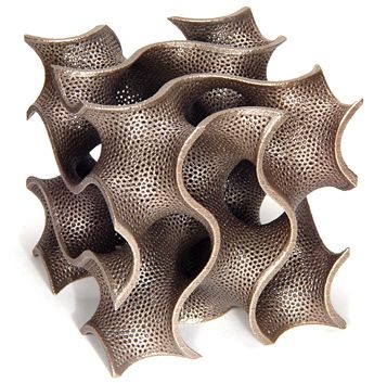
Mathematica to represent the curves as tubes with the given radius, the
         PlotPoints directive tells it the number of sides that the tubes are to have,
         and the PlotRange directive makes sure it doesn’t crop out any parts of
         the geometry.

       • The tubes that these lines generate are embedded closed polygonal meshes,
         see Figure 8a. These meshes intersect each other at grid intersections, so
         the union of the tubes is not embedded5 . At corners of the grid, we get
         an ugly gap as in Figure 8b, because each curve is thickened into a tube
         only along the perpendiculars to the direction of the curve. A true regular
         neighbourhood of the curve would also include a hemisphere around each
         endpoint of the curve. We fix this by adding in our own sphere, as in Figure
         8c, which is what line 10 in the code does.

       • Finally, line 11 shows all three sets of 3D graphics objects together in the
         same space, and line 12 exports the mesh corresponding to those objects to
         our STL file.

  (a) The “Tube” PlotStyle      (b) At a corner, these leave   (c) This can be fixed by
  directive produces closed     an ugly gap.                   adding a sphere at the cor-
  polygonal meshes.                                            ner.

           Figure 8: Adding spheres at the corners of the parametric patch.

3.4       Using a 3D printing service
The STL file we generated in the previous section is ready to upload to a 3D print-
ing service as is. There are a number of 3D printing services with international
reach, and many other local companies. One either uploads the file to the com-
pany’s website, or emails the file to them. At some point, you will need to specify
   5
    If you use a 3D printing service, they should be able to fix this problem automatically on
upload. If you are using your own 3D printer then you may have to do some more work, taking
the Boolean union of the tubes.

                                              8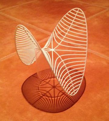
the units that the file is measured in, which is “millimetres” in our example, to be
consistent with our calculations in the Mathematica code.
    Some of the varieties of 3D printing technology are better suited to mathe-
matical models than others. In particular, many involve depositing two kinds of
material: the material that is to be the actual model, and a scaffolding material
that is broken off by hand after printing. This doesn’t work so well with an intri-
cate model with complicated internal structure. Other versions of the technology
use a dissolvable scaffolding material, or work by “solidifying” only the top layer
of a tank of dust, so the dust in lower layers supports the object as it is built.
Even given these restrictions, there is a large variety of available materials, ranging
from plastics to metals, glass and ceramics. Note however that different materials
have different requirements in terms of the minimum safe thickness of walls and
tubes and so on. The 3D printing service you use should have information avail-
able on their website or on request to help choose an appropriate technology and
material to print in. I usually use nylon plastic, 3D printed using a process called
“selective-laser-sintering” (often referred to as “SLS”). The material is inexpensive,
very strong, and is flexible rather than brittle. At the time of writing, the model
generated in this article cost me less than US$10 in this material.

                         Figure 9: The 3D printed object.

4    Going Further
There are an enormous number of interesting and beautiful mathematical models
that can be generated with Mathematica alone. For further inspiration, George
Hart has also written on using Mathematica to produce geometry suitable for 3D
printing [10]. However, for more complicated models, it may make more sense to
use a 3D design program, such as Rhinoceros or Blender, or one of the others listed

                                          9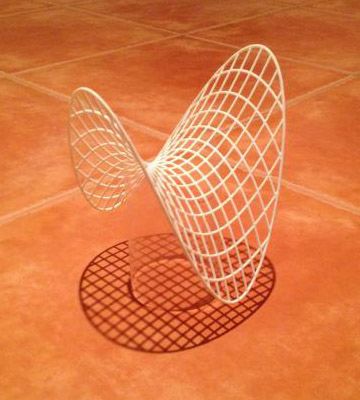
above. These allow a large amount of control over the 3-dimensional geometry,
and act in some ways like 3-dimensional versions of 2-dimensional vector graphics
programs, such as Adobe Illustrator, Inkscape or Xfig. One can move individual
parts of a model around, copy and paste, and transform objects in various ways.
The equivalent of the Mathematica “PlotStyle->Tube” directive lets us build tubes
around given curves, and one can build complicated mesh surfaces by joining
together parameterised patches. For more details, see http://www.segerman.
org/3d_printing_notes.html. Good luck!

References
 [1] Robert McNeel & Associates, Rhinoceros, http://www.rhino3d.com/.

 [2] Autodesk, 3ds max, http://usa.autodesk.com/3ds-max/.

 [3]          , Maya, http://usa.autodesk.com/maya/.

 [4] Vladimir Bulatov, Bulatov abstract creations, http://bulatov.org/.

 [5] ISTI CNR, MeshLab, http://meshlab.sourceforge.net/.

 [6] Blender Foundation, Blender, http://www.blender.org/.

 [7] Bathsheba Grossman, Bathsheba sculpture, http://www.bathsheba.com.

 [8] George W. Hart, The (10, 3)-a network, http://www.georgehart.com/rp/
     10-3.html.

 [9]           , Creating a mathematical museum on your desk, Mathematical Intel-
       ligencer 27 (2005), no. 4, 14–17.

[10]         , Procedural generation of sculptural forms, Proceedings of
       the Bridges Conference, also available at http://www.georgehart.com/
       ProceduralGeneration/Bridges08-Hart10pages.pdf, 2008.

[11] Jesse Louis-Rosenberg and Jessica Rosenkrantz, Nervous system, http://
     n-e-r-v-o-u-s.com/.

[12] Burkard Polster and Marty Ross, Print your own socks, Column in The Age,
     also available at http://education.theage.com.au/cmspage.php?intid=
     147&intversion=78, February 2011.

[13] Saul Schleimer and Henry Segerman, Sculptures in S 3 , submitted for publi-
     cation.

[14] Carlo Séquin, http://www.cs.berkeley.edu/~sequin/.

[15] Wolfram Research,        Inc.,   Mathematica,    http://www.wolfram.com/
     mathematica/.

                                        10
You can also read