Circuit Design and Experimental Investigations for a Predator-Prey Model - Exeley
←
→
Page content transcription
If your browser does not render page correctly, please read the page content below
INTERNATIONAL JOURNAL ON SMART SENSING AND INTELLIGENT SYSTEMS
Article | DOI: 10.21307/ijssis-2018-010                                                                       Issue 0 | Vol. 0

Circuit Design and Experimental Investigations for a
Predator-Prey Model
Afef Ben Saad, Ali Hmidet and
Olfa Boubaker
                                                Abstract
National Institute of Applied                   In recent years, dynamical relationship between species in ecology
Sciences and Technology, INSAT,                 has been intensively investigated and will continue to be one of the
Centre Urbain Nord BP. 676,
                                                most significant themes. The dynamics of predator–prey’s systems
1080 Tunis Cedex, Tunisia.
                                                are at the heart of these studies. Such models are generally depicted
E-mail: afef.ben.saad88@gmail.com,              by nonlinear polynomials and exhibit many complex nonlinear phe-
hmidetali@yahoo.fr,                             nomena. In this paper, not only a prey–predator model displaying
olfa.boubaker@insat.rnu.tn.                     richer dynamical behaviors is analyzed but also its electronic circuit
This article was edited by Tariqul              is also designed via the MultiSIM software proving the very good
Islam.                                          agreement between biological theory considerations and electronic
Received for publication January 12,            experiments.
2018.
                                                Keywords
                                                Circuit design, MultiSIM, experiments, predator–prey model.

Ecology is the study of interactions among organisms              attempt to reproduce the complex dynamics of such
and their environment. There are many useful applica-             systems using an equivalent electrical circuit. While,
tions of ecology as natural resource management and               certain biological systems such as biological tissue
city planning (Laktionov et al., 2017; Teay et al., 2017;         and biological neural network are modeled by electri-
Umar et al., 2017; Visconti et al., 2017). However, ecol-         cal circuit (Le Masson et al., 1999; Gómez et al., 2012).
ogy is also concerned by understanding and analyzing              As such predator–prey systems exhibit complex
the dynamical behavior of populations in ecosystem                dynamics as chaotic behaviors (Luo et al., 2016), such
in order to predict their undesired dynamics (Feng                circuits can be adopted in the future in communication
et al., 2017; Zhang et al., 2017b). On the other hand,            for encryption tasks (Lassoued and Boubaker, 2016;
understanding population dynamics are leading nowa-               Lassoued and Boubaker, 2017; Kengne et al., 2017).
days to many interesting optimization algorithms such                 In this paper, the predator–prey system, already
as Particle Swarm algorithms (Mehdi and Boubaker,                 analyzed in Ben Saad and Boubaker (2015, 2017),
2011, 2016;), Ant Colony algorithms (Pang et al., 2017;           and incorporating nonlinear polynomials in its complex
Yongwang et al., 2017) and Prey-predator algorithms               model is considered for the weak Allee Effect case
(Sidhu and Dhillon, 2017; Zhang and Duan, 2017).                  study. The objective is to design a suitable electronic
    It is obvious that it is not at all evident to construct a    circuit permitting to understand and conceptualize
mathematical model that will fit entirely any natural pop-        many aspects of ecological experimentation and theory
ulation interactions. In the literature, several models for       by using only simple analog electronic components.
predator–prey’s systems have been already proposed                It is clear that proving a good agreement between
and analyzed incorporating some specific effects                  biological theory and electronic experiments is not evi-
(Bürger et al., 2017; Elettreby et al., 2017; Li et al.,          dent due to the imperfections and uncertainties related
2017a, 2017b; Liu et al., 2017, 2018; Liu and Dai; Liu            to electronic components. Despite, these undesirable
and Wiang, 2018; Yuan et al., 2018; Zhang et al.,                 effects, the main nonlinearities of the biological model
2017a). The first proposed one was the Lotka Volterra             will be validated by means of experimental data. The
predator–prey model (Volterra, 1928). However, to the             circuit related to the prey–predator model will be then
best of our knowledge, there is no research work that             designed and simulated using the MultiSIM software.

© 2018 Authors. This work is licensed under the Creative Commons Attribution-Non-                                           1
Commercial-NoDerivs 4.0 License https://creativecommons.org/licenses/by-nc-
nd/4.0/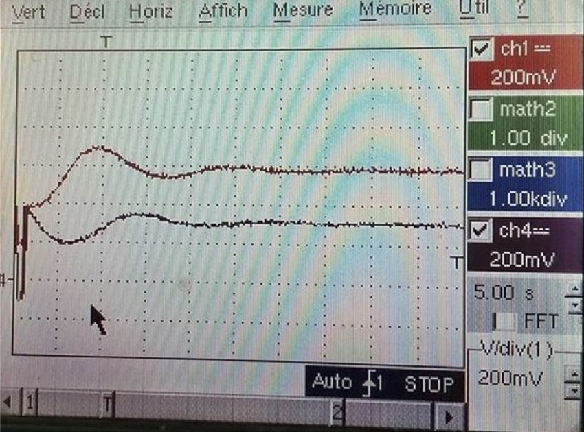
Circuit design and experimental investigations for a predator-prey model
This work is arranged as follows: Sections “PRED- For i = 1, …, 3, the corresponding Jacobian matrix
ATOR–PREY MATHEMATICAL MODEL” and “WEAK Ji and eigenvalues (λ1i, λ2i) are given by
ALLE EFFECT CASE STUDY ANALYSIS” recall the
nonlinear model as well as its basic dynamics. Then,
numerical simulation of the global dynamic behavior − 0 λ10 = −l (2)
J0 = and
of the system is presented in Section “NUMERICAL 0 −m λ20 = − m
SIMULATIONS VIA MATCONT SOFTWARE”. In Sec-
tion “EXPERIMENTAL VALIDATION OF MAIN NON-
LINEARITIES”, the circuit design, simulation results ( − 1) −1 λ11 = l − 1 (3)
J1 = and
via the MultiSIM software as well as the experimental 0 (1− m ) λ21 = 1− m
data of the main nonlinearities of the predator–prey
model are investigated. In Section “CIRCUIT DESIGN
VIA MULTISIM SOFTWARE”, the circuit design of
the whole complex model is finally proposed and a tr( J3 ) + i ∆
( −2 m2 + m( + 1)) − m λ12 =
good agreement between simulation results via MAT- 2 (4)
J3 = and
CONT and MultiSIM softwares are shown. Finally, ( m − )(1 − m) 0
λ = tr( J 3 ) − i ∆
an experimental implementation is illustrated in sec- 22 2
tion “EXPERIMENTAL IMPLEMENTATION OF THE
PREDATOR–PREY MODEL”.
with tr(J2) = m (ℓ + 1 − 2 m); Δ = [m (ℓ + 1 − 2 m)]2 − 4[m(m − ℓ)
(1 − m)].
Predator–Prey mathematical model Based on the last results, the singularities and the
phase portraits of the neighborhood of all equilibriums
Consider the predator–prey model with Allee Effect are summarized in Table 1.
described by Ben Saad and Boubaker, (2015, 2017):
dx1
dt = x1 ( x1 − )( k − x1 ) − x1 x 2 , Numerical simulations via
dx 2 = e ( x − m ) x , (1) matcont software
dt 1 2
The global dynamics of the system (1), already de-
where x1 is the size of the prey population and x2 the tailed in Table 1, will be proved numerically in this
size of the predator population, ℓ is the Allee Effect section using the Matcont software (Dhooge et al.,
threshold, k is the carrying capacity, e is the feeding 2008). Since the two first equilibriums E0 and E1 exist
efficiency of Lotka–Volterra model and m is the pred- ∀m ∈ [0 1], only the singularity of the equilibrium E3
ator mortality rate. Let consider also the biologically will be shown numerically in the following for the initial
meaningful conditions x1 ≥ 0 and x2 ≥ 0. condition (x1 = 0.4; x2 = 0.3). For m = −ℓ = 0.2, Figure 1
Two case studies for the Allee effect ℓ can be con- shows the temporal evolution of the dynamics of sys-
sidered (Dhooge et al., 2008): tem (1) whereas the phase portrait of the system is
shown in Figure 2.
• The Strong Allee effect when ℓ ∈ [0 1], As it is shown, a heteroclinic orbit appears indicat-
• The Weak Allee effect when ℓ ∈ [−1 0]. ing the existence of a global bifurcation described by
an attractor which bifurcates from an unstable focus
In the following, only the Weak Allee effect case equilibrium point to a heteroclinic cycle. The two pop-
study will be considered and the parameters k, e, and ulations’ dynamics oscillate between 0 and 1 density
m are taken as k = e = 1 and m ∈ [0 1]. values. Figures 3 and 4 show the dynamic behavior
of the system at the non-isolated point E3 (0.4, 0.36)
Weak alle effect case study analysis when m = 0.4.
For the second case study, the obtained behavior
For k = e = 1, ℓ ∈ [−1 0] and m ∈ [0 1], the system (1) of the two populations is periodic which is described
admits three equilibriums Ei(i = 1, …, 3): as a circle around the equilibrium E3 (0.4, 0.36). When
m = 0.6, the dynamic behavior of the system is shown
1. The zero equilibrium E0 = (0, 0), in Figures 5 and 6.
2. The two non-isolated equilibriums E1 = (ℓ, 0), The obtained phase portrait shows a stable
3. The equilibrium E2 = (m, (m − ℓ) (1 − m)). focus. This latter closes to a fixed point with the
2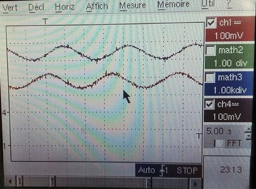
INTERNATIONAL JOURNAL ON SMART SENSING AND INTELLIGENT SYSTEMS

Table 1. Predator–prey model analysis.

Equilibrium       Singularities    Phase portraits

E0 (0,0) Re(λ1)
                  Saddle point
≥ 0, Re(λ2) ≤ 0

E1 (1,0) Re(λ1)
                  Saddle point
≥ 0, Re(λ2) ≤ 0

                                   m = 0.4 Re(λ1) = Re(2) = 0

E2 (m, (m−ℓ)
                  m = 0.4
(1−m)) Im(λ1)
                  Center
≥ 0, Im(λ2) ≤ 0

                                   m  0.4 Re(λ1) = Re(λ2) ≤ 0

                  m > 0.4
                  Stable focus

                                                                                                       3
Circuit design and experimental investigations for a predator-prey model

               Figure 1: Temporal evolution of the predator–prey system for m = 0.2: (A) prey and (B) predator.

                                                              following coordinates (0.6, 0.32) proven with the tem-
                                                              poral evolution.

                                                              Experimental validation
                                                              of main nonlinearities
                                                              The aim of this section is to design an analog
                                                              circuit that can build the nonlinear terms according
                                                              to system (1). Therefore, equivalent electronic circuits
                                                              of these nonlinear terms are designed and simulated
                                                              via MultiSIM software (Yujun et al., 2010). Due to
                                                              the complexity of the equivalent circuit design, we
                                                              designed first the equivalent circuit of each nonlinear
               Figure 2: Phase portrait of the                term x2 and x3. The first nonlinear term circuit needs
               predator–prey system for m = 0.2.              one Multiplier AD6333. The multiplying core of this

               Figure 3: Temporal evolution of the predator–prey system for m = 0.4: (A) prey and (B) predator.

4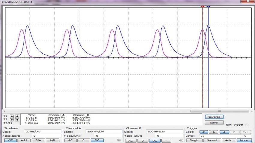
INTERNATIONAL JOURNAL ON SMART SENSING AND INTELLIGENT SYSTEMS
Figure 4: Phase portrait of the Figure 6: Phase portrait of the
predator–prey system for m = 0.4. predator–prey system for m = 0.6.
multiplier comprises a buried Zener reference providing
( R3 + R4 ) x x 2 ( R1 + R2 ) ( R3 + R4 ) x
an overall scale factor of 10 V. For that, an amplification S2 = x 3 = S1 =
R3 10 10 R1 R3 10
of the output with a gain of 10 is required. Thus, the
equivalent electrical model of x2 is realized as follows: ( R1 + R2 )( R3 + R4 ) x 3
=
R1R3 100
x 2 ( R1 + R2 )
S1 = x 2 = .
10 R1 The input which will be used for the equivalent
circuit of system (1) is continuous. However, in this part,
As shown in Figure 7, by considering the compo- in order to verify the efficiency of the two nonlinear
nents datasheet, the electronic circuit of the nonlinear terms equivalent circuits, an alternative signal is used
term x2 is modeled by one Analog multiplier AD633AN, as an input with a weak frequency equal to 1 Hz and
one Amplifier AOP, two capacitors (C1, C2) and two re- amplitude of 2 V. The square and the cube of the signal
sistors (R2, R2). Due to the existence of internal loss in are presented with a pink curve in Figure 9 and Figure 10,
the electrical components, the ideal value of R2 chosen respectively. For high frequencies (1 kHz, 10 kHz,
to obtain the best result is 0.9 kΩ. However, for the non- 100 kHz), we obtained the same following results.
linear term x3, the electronic circuit is modeled in Figure 8 As it is shown, we have chosen the same scale for
by two multipliers AD633AN, 2 Amplifiers AOP, four the two nonlinearities. For the first nonlinearity x2, the
capacitors and four resistors, since its electrical model obtained signal amplitude is equal to 4,108 V which
is realized as follows: obviously the square of the input signal amplitude.
Figure 5: Temporal evolution of the predator–prey system for m = 0.6: (A) prey and (B) predator.
5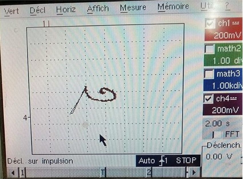
Circuit design and experimental investigations for a predator-prey model

               Figure 7: Circuit design of the x2 function within MultiSIM software.

In addition, for the second nonlinearity x3, the result       numerical simulations with Matlab, the electrical
proves that the obtained signal is the cubes of the           simulations with MultiSIM and the experimental
input signal since the obtained amplitude is equal to         results for the two nonlinearities.
7,980 V which is almost equal to 8 V the cube of the
input amplitude.
    Figures 11 and 12 show an experimental imple-             Circuit design via multisim software
mentation for the last simulation results. The oscillo-
scope traces of the proposed circuit are illustrated in       In this section, the agreement between biological theory
Figures 13 and 14.                                            and electronic experiments of the predator–prey model
    Comparing the different results, it is proven that        will be analyzed by considering the three cases studies
there is a good qualitative agreement between the             presented numerically by MATCONT. Therefore, a trans-

               Figure 8: Circuit design of the x3 function within MultiSIM software.

6
INTERNATIONAL JOURNAL ON SMART SENSING AND INTELLIGENT SYSTEMS
Figure 9: Simulation results of the x2 function with MultiSIM Software.
Figure 10: Simulation results of the x3 function with MultiSIM Software.
formation of the biological predator–prey model (1) to an 1 1 1 1 1
where = = = 1, = (1+ I); = I,
equivalent electrical model is realized as follows: C1R1 C1R4 C2 R5 C1R2 C2 R3
dx1 1 1 1 1 1
3 2 = m C and C2 are used for the integration of
dt = C R x1 + C R x1 − C R x1 − C R x1 x2 C2 R6 1
1 1 1 2 1 3 1 4
the circuit outputs in order to obtain as output the
dx 1 1
2
= xx − x , populations’ density x1 and x2.
dt C2 R5 1 2 C2 R6 2 (5)
7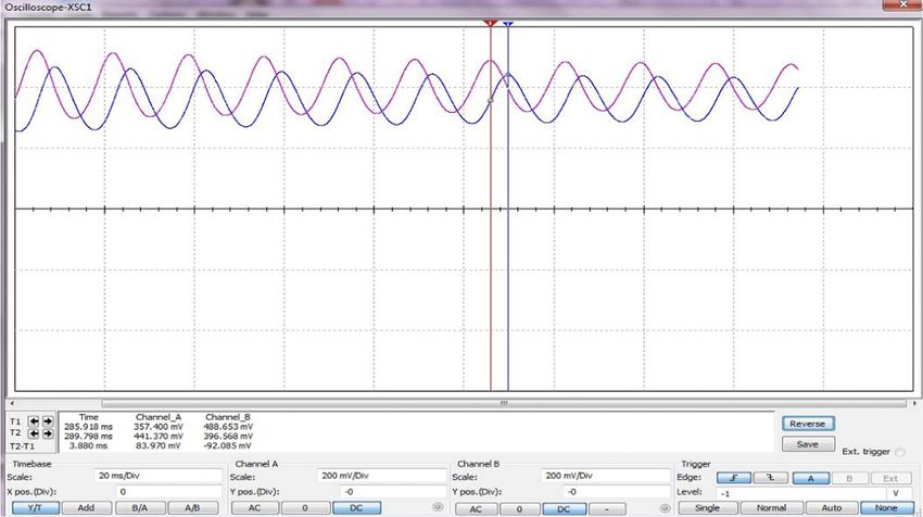
Circuit design and experimental investigations for a predator-prey model

                                                                             Figure 13: Experimental results of x2
               Figure 11: Electronic circuit of the x2                       function.
               function.

    The electronic circuits corresponding to these            the amplitude of the blue and pink curves are
cases are designed by the software MultiSIM and               almost equal to 0.956 V and 0.836 V, respectively.
presented in the following. We have used three multi-         Comparing with the numerical simulation present-
pliers, five AOP, two capacitors and 12 resistors. The        ed in Figures 1 and 2, we conclude that the per-
resistors (R1, R2, …, R6) and capacitors values are           manent regime of the system dynamic obtained
fixed with respect to the parameters values. The val-         via MultiSIM is similar to that obtained using the
ue of the two capacitors C1 and C2 is fixed at 100 nF.        Matcont software.
In addition, two interrupters S1 and S2 are used to in-            In the second case study, we consider the mor-
troduce the initial conditions of the prey and predator       tality rate of the predator m = 0.4. Thus, Figure 18
density. In order to analyze the three case studies, we       describes the electrical circuit of the model with
vary the value of the resistor R6 which corresponds to        R6 = 25 k Ω . Then, the temporal evolution and the
                              R5                              phase portrait are illustrated in Figure 19 and Figure 20,
the parameter m since R6 = m . In the first case study,
                                                              respectively.
we consider the mortality rate of the predator m = 0.2.
Therefore, the fixed value of R6 in this case is equal to          As it is illustrated in the temporal evolution,
50 k Ω . Figure 15 describes the electrical circuit of the    the maximum amplitude of the prey population
predator–prey model (5).                                      is equal to 0.488 V and that of the predator pop-
   Then, the temporal evolution and the phase                 ulation is equal to 0.441 V. The obtained values
portrait when m = 0.2 are presented in Figure 16 and          are obviously very close to the numerical values
Figure 17, respectively.                                      shown in Figure 3. Furthermore, the phase por-
   We obtained two phase-shifted alternative                  trait proves the existence of the center singularity
signals. The pink curve corresponds to the dynamic            which is demonstrated numerically via the Matcont
evolution of the prey while the blue one corresponds          software in Figure 4.
to the dynamic evolution of the predator. Based                    In the third case study, the mortality rate of
on the scale chosen in the temporal evolution,                the predator m is fixed at 0.6. Therefore, Figure 21

               Figure 12: Electronic circuit of the x3                       Figure 14: Experimental results of x3
               function.                                                     function.

8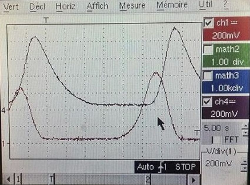
INTERNATIONAL JOURNAL ON SMART SENSING AND INTELLIGENT SYSTEMS

Figure 15: Circuit design of the predator–prey system for m = 0.2.

Figure 16: Temporal evolution via MultiSIM software (m = 0.2).

                                                                                            9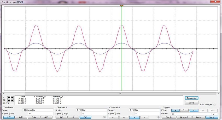
Circuit design and experimental investigations for a predator-prey model

               Figure 17: Phase portrait via MultiSIM software (m = 0.2).

               Figure 18: Circuit design of the predator–prey system for m = 0.4.

10
INTERNATIONAL JOURNAL ON SMART SENSING AND INTELLIGENT SYSTEMS
Figure 19: Temporal evolution via MultiSIM software (m = 0.4).
Figure 20: Phase portrait via MultiSIM software (m = 0.4).
presents the electrical circuit with R6 = 17 kΩ . Figures results. The obtained temporal evolution and phase
22 and 23 illustrate the corresponding temporal evo- portrait prove that the model dynamic tends toward
lution and phase portrait. a fixed point. In Figure 22, it is noted that the dynamic
For the third case study, we change slightly the behavior oscillates during the transitional regime,
=
initial conditions =
( x1 0.4, x 2 0.1) to obtain the clearest whereas in the permanent regime, it becomes
11Circuit design and experimental investigations for a predator-prey model
Figure 21: Circuit design of the predator–prey system for m = 0.6.
Figure 22: Temporal evolution via MultiSIM software (m = 0.6).
12INTERNATIONAL JOURNAL ON SMART SENSING AND INTELLIGENT SYSTEMS
Figure 23: Phase portrait via MultiSIM software (m = 0.6).
Figure 25: Experimental temporal
evolution (m = 0.2).
a pick of 0.978 V. However, the blue curve
corresponding to the predator population reaches
a pick equal to x2 = 0.399 V. This temporal behav-
ior is described by a stable focus in the obtained
Figure 24: STM3278 Technology. phase portrait. These electrical results are almost
similar to the numerical ones presented in Figures
5 and 6.
continuous reaching a constant value equal to For the three cases study, we conclude that the
0.586 V for the prey population and to 0.326 V for electrical results obtained by the software MultiSIM
the predator one. The pink curve correspond- obviously prove the numerical results obtained by the
ing to the prey population dynamic reaches Matcont software.
13Circuit design and experimental investigations for a predator-prey model
Figure 26: Experimental phase portrait Figure 28: Experimental phase portrait
(m = 0.2). (m = 0.4).
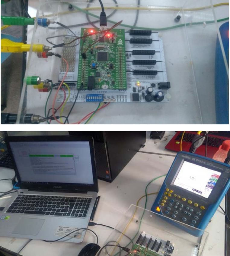
Experimental implementation The experimental results of the three cases stud-
ies are obtained by using the oscilloscope and pre-
of the predator–Prey model sented in Figures 25–30.
In this section, an experimental implementation of the Comparing experimental results with numerical
equivalent electrical circuit will be realized by placing results obtained via the MATCONT software shown in
the different electrical components on a bread board Figures 1–6, we can conclude that good agreement is
within the laboratory. obtained between simulation results and experiments.
As it is mentioned previously, mathematical pred-
ator–prey model has several nonlinearities which are Conclusion
modeled by multipliers AD633 in the equivalent elec-
trical circuit. The cascade of components AD633 and In this paper, an electronic circuit is designed for the
AOP with gain of 10 amplifies most likely the imper- model of a prey–predator model and its complex be-
fection and the uncertainties of the electronic com- havior is proved via numerical and electrical results.
ponents and consequently distorts the experimental Furthermore, some experimental investigations are
results. Therefore, in order to resolve this problem, also shown and demonstrate that they can be used
the experimental validation is realized by using the to characterize the ecological dynamics faster. In the
technology STM3278 shown in Figure 24. future, we will try to prove, via experimental results,
Figure 27: Experimental temporal Figure 29: Experimental temporal
evolution (m = 0.4). evolution (m = 0.6).
14INTERNATIONAL JOURNAL ON SMART SENSING AND INTELLIGENT SYSTEMS
Gómez, F., Bernal, J., Rosales, J., and Cordova, T.
2012. Modeling and simulation of equivalent circuits in
description of biological systems–a fractional calculus
approach. Journal of Electrical Bioimpedance 3: 2–11.
Kengne, J., Jafari, S., Njitacke, Z.T., Khanian,
M.Y.A., and Cheukem, A. 2017. Dynamic analysis and
electronic circuit implementation of a novel 3D auton-
omous system without linear terms. Communications
in Nonlinear Science and Numerical Simulation 52:
62–76.
Laktionov, I.S., Vovna, O.V., and Zori, A.A. 2017.
Planning of remote experimental research on effects
of greenhouse micriclimate parameters on vegetable
crop-producing. International Journal on Smart Sens-
ing and Intelligent Systems 10(4): 845–62.
Figure 30: Experimental phase portrait Lassoued, A., and Boubaker, O. 2016. On new chaotic
(m = 0.6). and hyperchaotic systems: a literature survey. Nonlinear
Analysis: Modelling and Control 21(6): 770–89.
the chaotic dynamics of such nonlinear systems in Lassoued, A., and Boubaker, O. 2017. Dynamic
the presence of seasonally effects in order to use analysis and circuit design of a novel hyperchaotic
such circuits for encryption/decryption fields. system with fractional-order terms. Complexity 2017.
Le Masson, S., Laflaquerie, A., Bal, T., and Le
Masson, G. 1999. Analog circuits for modeling bio-
Literature Cited logical neural networks: design and applications. IEEE
Transactions on Biomedical Engineering 46(6).
Ben Saad, A., and Boubaker, O. 2015. On bifur- Li, H.L., Zhang, L., Hu, C., Jiang, Y.L., and Teng, Z.
cation analysis of the predator–prey BB-model with 2017b. Dynamical analysis of a fractional-order pred-
weak allee effect. IEEE 16th international conference ator–prey model incorporating a prey refuge. Jour-
on Sciences and Techniques of Automatic Control and nal of Applied Mathematics and Computing 54(1–2):
Computer Engineering, Monastir, 19–23. 435–49.
Ben Saad, A., and Boubaker, O. 2017. A new fractional- Li, M., Chen, B., and Ye, H. 2017a. A bioeconomic dif-
order predator–prey system with allee effect, in Azar, ferential algebraic predator–prey model with nonlinear
A.T., Vaidyanathan, S., and Ouannas, A. (eds), Fractional prey harvesting. Applied Mathematical Modelling 42:
Order Control and Synchronization of Chaotic Systems 17–28.
688, Springer, Berlin, 857–77. Liu, G., Wang, X., Meng, X., and Gao, S. 2017.
Bürger, R., Ruiz-Baier, R., and Tian, C. 2017. Stabil- Extinction and persistence in mean of a novel delay im-
ity analysis and finite volume element discretization for pulsive stochastic infected predator–prey system with
delay-driven spatio-temporal patterns in a predator– jumps. Complexity 2017.
prey model. Mathematics and Computers in Simulation Liu, M., He, X., and Yu, J. 2018. Dynamics of a sto-
132: 28–52. chastic regime-switching predator–prey model with
Dhooge, A., Govaerts, W., Kuznetsov, Y.A., Meijer, harvesting and distributed delays. Nonlinear Analysis:
H.G.E., and Sautois, B. 2008. New features of the Hybrid Systems 28: 87–104.
software MatCont for bifurcation analysis of dynami- Liu, W., and Wiang, Y. 2018. Bifurcation of a delayed
cal systems. Mathematical and Computer Modelling of gause predator–prey model with michaelis-menten
Dynamical System 14: 147–75. type harvesting. Journal of Theoretical Biology 438:
Elettreby, M.F., Al-Raezah, A.A., and Nabil, T. 2017. 116–32.
Fractional-Order Model of Two-Prey one-predator Liu, X., and Dai, B., Dynamics of a predator–prey
system. Mathematical Problems in Engineering 2017. model with double allee effects and impulse. Nonlinear
Feng, X., Shi, K., Tian, J., and Zhang, T. 2017. Ex- Dynamics 88(1): 685–701.
istence, multiplicity, and stability of positive solutions Luo, Z., Lin, Y., and Dai, Y. 2016. Rank one chaos in
of a predator–prey model with dinosaur functional re- periodically kicked lotka-volterra predator–prey system
sponse. Mathematical Problems in Engineering 2017. with time delay. Nonlinear Dynamics 85: 797–811.
15Circuit design and experimental investigations for a predator-prey model
Mehdi, H., and Boubaker, O. 2011. Position/force International Journal on Smart Sensing and Intelligent
control optimized by particle swarm intelligence for Systems 10(1): 18–49.
constrained robotic manipulators. In IEEE 11th Inter- Volterra, V. 1928. Variations and fluctuations of the
national Conference on Intelligent Systems Design number of individuals in animal species living together.
and Applications (ISDA), Nov. 22–24, 2011, Cordoba, ICES Journal of Marine Science 3(12): 3–51.
Spain, 190–195. Yongwang, L., Yu-ming, L., Heng-bin, Q., and Yan-
Mehdi, H., and Boubaker, O. 2016. PSO-Lyapunov feng, B. 2017. A new mathematical method for solving
motion/force control of robot arms with model uncer- cuttings transport problem of horizontal wells: ant colony
tainties. Robotica 34(3): 634–51. algorithm. Mathematical Problems in Engineering 2017.
Pang, S., Zhang, W., Ma, T., and Gao, Q. 2017. Ant Yuan, H., Wu, J., Jia, Y., and Nie, H. 2018. Coex-
colony optimization algorithm to dynamic energy man- istence states of a predator–prey model with cross-
agement in cloud data center. Mathematical Problems diffusion. Nonlinear Analysis: Real World Applications
in Engineering 2017. 41: 179–203.
Sidhu, D.S., and Dhillon, J.S. 2017. Design of digital Yujun, N., Xingyuan, W., Mingjun, W., and
IIR filter with conflicting objectives using hybrid pred- Huaguang, Z. 2010. A new hyperchaotic system and
ator–prey optimization. Circuits, Systems, and Signal its circuit implementation. Communication in Nonlinear
Processing, 1–25. Science and Numerical Simulation 15: 3518–24.
Teay, S.H., Batunlu, C., and Albarbar, A. 2017. Zhang, B., and Duan, H. 2017. Three-dimensional
Smart sensing system for enhancing the reliability of path planning for uninhabited combat aerial vehicle
power electronic devices used in wind turbines. Inter- based on predator–prey pigeon-inspired optimiza-
national Journal on Smart Sensing and Intelligent Sys- tion in dynamic environment. IEEE/ACM Transactions
tems 10(2): 407–24. on Computational Biology and Bioinformatics (TCBB)
Umar, L., Setiadi, R.N., Hamzah, Y., and Linda, T.M. 14(1): 97–107.
2017. An Arduino Uno based biosensor for watter pol- Zhang, L., Liu, J., and Banerjee, M. 2017a. Hopf and
lution monitoring using immobilized Algae Chlorella Vil- Steady state bifurcation analysis in a ratio-dependent
garis. International Journal on Smart Sensing and Intel- predator–prey model. Communications in Nonlinear
ligent Systems 10(4) 955–75. Science and Numerical Simulation 44: 52–73.
Visconti, P., Primiceri, P., de Fazio, R., and Ekuak- Zhang, X., Li, Y., and Jiang, D. 2017b. Dynamics
ille, A.L. 2017. A solar-powered white led-based UV- of a stochastic holling type II predator–prey model
VIS spectrophotometric system managed by PC for air with hyperbolic mortality. Nonlinear Dynamics 87(3):
pollution detection in faraway and unfriendly locations. 2011–20.
16You can also read