Comparison of Background Subtraction Techniques Under Sudden Illumination Changes
←
→
Page content transcription
If your browser does not render page correctly, please read the page content below
Comparison of Background Subtraction Techniques
       Under Sudden Illumination Changes
                                       C.J.F. Reyneke, P.E. Robinson and A.L. Nel
                              Department of Electrical and Electronic Engineering Science
                                    Faculty of Engineering and the Built Environment
                                                University of Johannesburg
                              email: corius.reyneke@gmail.com; {philipr, andren}@uj.ac.za

   Abstract—This paper investigates three background modelling       pixel order values in local neighbourhoods are preserved in
techniques that have potential to be robust against sudden and       the presence of sudden illumination changes. They provide
gradual illumination changes for a single, stationary camera. The    an output image by classifying each pixel by its probability
first makes use of a modified local binary pattern that considers
both spatial texture and colour information. The second uses a       of order consistency [3]. Pilet et al. make use of texture
combination of a frame-based Gaussianity Test and a pixel-based      and colour ratios to model the background and segment the
Shading Model to handle sudden illumination changes. The third       foreground using an expectation-maximization framework [4].
solution is an extension of a popular kernel density estimation      Texture-based features work well, but only in scenes with
(KDE) technique from the temporal to spatio-temporal domain          sufficient texture; untextured objects prove to be a difficulty.
using 9-dimensional data points instead of pixel intensity values
and a discrete hyperspherical kernel instead of a Gaussian kernel.      Another way of dealing with sudden illumination changes
   A number of experiments were performed to provide a com-          is to maintain a representative set of background models [5].
parison of these techniques in regard to classfication accuracy.     These record the appearance of the background under differ-
   Index Terms—background subtraction, sudden illumination           ent lighting conditions and alternate between these models
changes.                                                             depending on observation. The techniques that make use of
                                                                     this approach mostly differ in their method of deciding which
                      I. I NTRODUCTION                               model should be used for the current observation. Toyama
   Background subtraction techniques have traditionally been         et al. [6], implement the Wallflower system which chooses
applied to object detection in computer vision systems and           the model as the one that produces the lowest number of
have since become a fundamental component for many appli-            foreground pixels. This proves to be an unreliable criterion
cations ranging from human pose estimation to video surveil-         for real-world scenes. Stenger et al. [7] make use of hidden
lance. The goal is to remove the background in a scene so            Markov models but in most cases, sharp changes occur without
that only the interesting objects remain for further analysis or     any discernible pattern. Also, Stenger et al. and Toyama et al.
tracking. Techniques such as these are especially useful when        require off-line training procedures and consequently cannot
they can identify object regions without prior information and       incorporate new real-world scenes into their models during
when they can perform in real-time.                                  run-time [8]. Sun [9] implements a hierarchical Gaussian
   Real-life scenes often contain dynamic backgrounds such as        Mixture Model (GMM) in a top-down pyramid structure. At
swaying trees, rippling water, illumination changes and noise.       each scale-level a mean pixel intensity is extracted and is
While a number of techniques are effective at handling these,        matched to the best model of its upper-level GMM. While
sudden illumination changes such as a light source switching         mean pixel intensity is useful for the detection of illumi-
on/off or curtains opening/closing continue to be a challenging      nation changes, it is also sensitive to changes caused by
problem for background subtraction [1]. In recent years a            the foreground. Additionally, the Hierarchical GMM does
number of new segmentation techniques have been developed            not exploit any spatial relationships among pixels which can
that are robust to sudden illumination changes but only for          output incoherent segmentation [5]. Dong et al. [10] employ
certain scenes. Our aim is to eventually identify the best-          principle component analysis (PCA) to build a number of
performing solution, improve upon it, and implement it on            subspaces where each represent a single background appear-
a GPU for real-time application.                                     ance. The foreground is segmented by selecting the subspaces
                                                                     which produces minimum reconstruction error. However, their
                     II. R ELATED W ORK                              work does not discuss how the system reacts to repetitive
   A number of texture-based methods have developed to               background movements.
solve the problem of sudden illumination changes. Heikkila              More recently, Zhou et al. [11], Ng et al. [1] and Vemu-
[2], Xie et al. [3] and Pilet et al. [4] make use of robust          lapalli [12] have developed techniques that have potential to
texture features [5]. Heikkila makes use of local binary pattern     handle, and even be robust to, sudden illumination changes.
histograms as background statistics. Xie et al. assumes that         These will be discussed in more detail in section III.

                                                                 298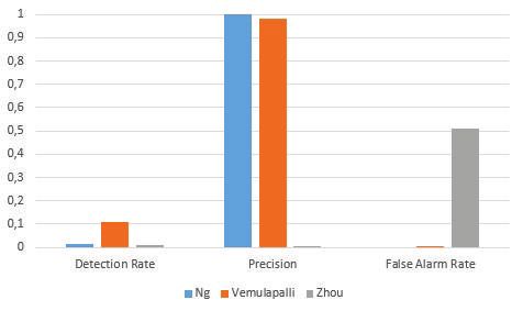
III. P ROPOSED S OLUTIONS current frame. If at least one proximity measure is above the
A. Background Modeling using Spatial-Colour Binary Pat- threshold then only the background histogram that produced
terns (SCBP) the highest proximity measure is updated using the following
formula:
This approach makes used of a novel feature extraction m̄k = αb h̄ + (1 − αb )m̄k (6)
operator, the Spatial-Colour Binary Pattern (SCBP), which
takes spatial texture and colour information into consideration Where m̄k is the model SCBP histogram, h¯k is the current
[11]. It is an extension of a local binary pattern which is frame SCBP histogram and αb is a learning rate such that
adapted to be centre-symmetrical and to consider only two αb ∈ [0, 1].
colour channels for the sake of computational efficiency. For Furthermore, the weights of the model are updated as
the sake of simplicity all processes relating to this solution follows:
apply to a single pixel and are performed on all the pixels in wk = αw Mk + (1 − αw )wk (7)
an image. Where αw is a learning rate such that αw ∈ [0, 1] and Mk is
SCBP2N,R (xc , yc ) = CSLBP2N,R (xc , yc ) 1 for the best-matching histogram and 0 for the rest.
Tp is an adaptive threshold that is maintained (for each
+2N +1 f (Rc , Gc |γ) + 2N +2 f (Gc , Bc |γ) (1)
pixel). The advantage of this is that static regions become
more sensitive while dynamic regions have a higher tolerance.
1, a > γb
f (a, b|γ) = (2) The threshold is updated as follows:
0, otherwise
Tp (x, y) = αp (s(x, y) − 0.05) + (1 − αp )Tp (x, y) (8)
Where Rc , Gc and Bc are the three colour channels of the
centre pixel (xc , yc ) and γ > 1 is a noise suppression factor. Where αp is a learning rate such that αp ∈ [0, 1] and s(x, y)
The Centre-Symmetrical Local Binary Pattern (CSLBP) is is a similarity measure of the highest value between the
defined as: current frame’s SCBP histogram bins and those of the model
N −1 histograms.
In order to determine the foreground mask the value for n
X
CSLBP2N,R (xc , yc ) = 2i s(gi − gi+N ) (3)
i=0 in the following equation is first determined.
w0 + w1 + ... + wn ≤ Tw (9)
1, x >= 0
s(x) = (4) Where the weights have been sorted into descending order.
0, x= ξstdi ]&[di /ḡi ≥ ε1 ],
measures are below the threshold, Tp , the model histogram Ωi = 1, if||(ri , gi , bi ) − (r̄i , ḡi , b̄i )||2 ≥ ε2 , (10)
with the lowest weight has its bins replaced with those of the 0, otherwise
299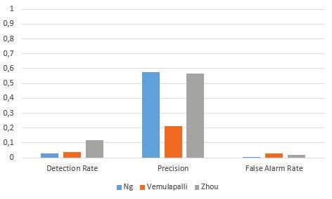
Where di = abs(gi − ḡi ) is the absolute deviation of intensity        change between two frames, such as a moving object, then
from the average and r, g and b are chromaticity coordinates            the ratio of pixel intensities will be constant and independent
calculated by r = R/(R + G + B), g = G/(R + G + B) and                  of the shading coefficients of the frames:
b = B/(R + G + B). The parameters ξ, ε1 and ε2 are tuning
                                                                                                        I1 (x, y)   Li,1
parameters.                                                                                 R(x, y) =             =                  (16)
   Finally, the average and standard deviation of the resulting                                         I2 (x, y)   Li,2
background pixels are updated as follows:                                  Under this assumption, if no foreground objects exist in
                                                                        a difference frame, the ratio of pixel intensities should re-
                    g¯i = βgi + (1 − β)g¯i                      (11)
                    q                                                   main constant and therefore be Gaussian distributed. Now, by
              stdi = β(gi − g¯i )2 + (1 − β)std2i               (12)    employing the shading model as an input to the Gaussianity
                                                                        test module, the background model can be made robust to
Where β is a learning rate such that β ∈ [0, 1] The chromatic-          sudden illumination changes. The equation used to generate
ity coordinates, r¯i , g¯i , b¯i , are updated in the same way as was   the moments used in the Gaussianity Test statistic is modified
done for g¯i .                                                          to make use of the pixel intensity ratio:
                                                                                               M −1        M −1
B. Background Modeling using a Shading Model and a Gaus-                                        2           2
                                                                                       1
                                                                          Jˆk (x, y) = 2
                                                                                               X           X
sianity Test                                                                                                      [Rgt (x+m, y+n)]k (17)
                                                                                      M
   The method proposed by Ng et al implements a hierarchical                                m=− M2−1 n=1− M2−1
framework that uses a combination of a pixel-based Shading
                                                                        Where
Model and a block-based Gaussianity Test [1]. This approach                                                BMt−1 (x, y)
is based on the assumption that camera noise is both spatially                              Rgt (x, y) =                             (18)
                                                                                                            It (x, y)
Gaussian, and temporally uncorrelated. If the difference of two
consecutive frames are taken, only Gaussian noise and fore-                The foreground mask is obtained using the following equa-
ground objects should remain. Under these assumptions, they             tions:
deduce that background pixels will be Gaussian distributed and                      Dt (x, y) = |It (x, y) − BMt−1 (x, y)|      (19)
foreground pixels will be non-Gaussian distributed. Therefore
background pixels can be distinguished from foreground pixels
                                                                                            foreground,        if Dt (x, y) > Ta
using a Gaussianity test.                                                    (x, y) ⊂                                                (20)
                                                                                            background,        otherwise
   The Gaussianity Test statistic is defined as follows:
                                                                        Where BMt (x, y) is the intensity value of the background
               H(J1 , J2 , J4 ) = J4 + 2J14 − 3J22              (13)    model at the coordinates (x, y) and time t, It (x, y) is the
Where Jk is a moment defined by the following equation:                 intensity value of the current pixel at the coordinates (x, y)
                      M −1       M −1
                                                                        and time t and Ta is an adaptive threshold. This equation is
              1        2          2                                     only employed in the foreground blocks as classified by the
 Jˆk (x, y) = 2
                      X          X
                                          [Dt (x + m, y + n)]k (14)     Gaussianity test.
             M
                   m=− M2−1   n=1− M2−1                                    Ta is an adaptive threshold which is calculated using an
   The Gaussianity Test statistic is expected to be close to            automatic, iterative method first proposed by Ridler [14]. This
zero when a set of samples is Gaussian distributed. If a set            method is computationally inexpensive but has the disadvan-
of samples in a block of size M xM has a Gaussianity Test               tage of assuming that the scene is bimodal. This assumption
statistic that is greater than a predefined threshold, τ , then the     predicts that there will be two distinct brightness regions in the
block is considered to contain foreground pixels.                       image represented by two peaks in the grey-level histogram
                                                                       of the input image. These regions correspond to the object
                       foreground,       if H > τ                       and its surroundings and so it is then reasonable to select the
          block =                                              (15)
                       background,       otherwise                      threshold as the grey-level half-way between these two peaks.
However, this assumption does not perform well in the pres-                The histogram of the current frame, It (x, y) is segmented
ence of sudden illumination changes. A shading model is                 into two parts using a threshold, Titerate , which is first set to
implemented to handle these.                                            the middle value (127) of the range of intensities. For each
   Ng et al extend the Gaussianity test with a shading model            iteration, the sample means of the foreground pixel intensities
proposed by Skifstad [13] in order to make it robust to sudden          and the sample means of the background pixel intensities are
illumination changes. The shading model is necessary because            calculated and a new threshold is determined as the average
the previous assumption that background regions are Gaussian            of these two means. The iterations stop once the threshold
distributed does not hold true in the presence of sudden                converges on a value, normally within about 4 iterations. The
illumination changes.                                                   following formula describes this process:
   The shading model assumes that a pixel intensity can                                      PTk              PN
                                                                                                b=0 bn(b)        b=T    bn(b)
be decomposed into an illumination value and a shading                              Tk+1 = PTk             + PN k+1                   (21)
coefficient. It is also assumed that if there is no physical                                2 b=0 n(b) 2 b=Tk+1 n(b)

                                                                    300
Where Tk is the threshold at the k th iteration, b is the intensity The N − 1 binary outputs of this module are then summed
value and n(b) is the number of occurrences of the value b in to produce a type of confidence measure, M of whether the
the image such that 0 ≤ b ≤ N . current pixel belongs to the background. This sum is then
Once the foreground mask has been segmented, morpho- thresholded using a value, T :
logical filtering is performed on the foreground mask in order M
to remove noise. Ng et al. perform one closing operation ≤T (25)
N
followed by one opening operation. The long-term and short-term models are updated using a
The values of the background pixels are updated using the blind update and selective update mechanism respectively. The
following formula: blind update adds a new 9-dimensional data point, Fi (x, y),
BMt (x, y) = to the sample set regardless of whether it belongs to the
background or foreground while the selective update adds the
data-point only if it belongs to the background. When a new
BMt−1 (x, y), if Dt (x, y) ≥ Ta
data point is added the oldest data point is removed from the
It (x, y), if Dt (x, y) < Tf
(22) sample set. The output of both the long-term and short-term
αIt (x, y)+
models are used as inputs to the foreground detection module.
(1 − α)BMt−1 (x, y), if Tf ≤ Dt (x, y) < Ta
The output of the module is described by the following table:
Where Tf is fixed and smaller than Ta and α is a learning
Long-term model Short-term model Output
rate such that ∈ [0, 1] Ol (x, y) = 0 Os (x, y) = 0 Of d (x, y) = 0
Ol (x, y) = 0 Os (x, y) = 1 Of d (x, y) = Of′ d (x, y)
C. Background Modeling using Non-parametric Kernel Den- Ol (x, y) = 1 Os (x, y) = 0 Of d (x, y) = 0
sity Estimation Ol (x, y) = 1 Os (x, y) = 1 Of d (x, y) = 1
The solution proposed by Vemulapalli is an extension of TABLE I: The output of the foreground detection module
the popular kernel density estimation (KDE) technique first which combines the output of the short-term and long-term
proposed by Elgammal et al. [15]. They extend the background background models.
model from the temporal to spatio-temporal domain by using
3x3 blocks centred at each pixel as 9-dimensional data points Where Ol (x, y) = 1 is the output of the long-term model,
instead of individual pixel intensity values [12]. In order to Os (x, y) = 1 is the output of the short-term model and
overcome the obvious increase in computational complexity Of d (x, y) = 1 is the output of the foreground detection
that this would cause, a hyper-spherical kernel is used instead module where:
of the typical Gaussian kernel. Each pass of the background P1 P1
1, if i=−1 j=−1
modeling module entails comparing the data points of the
Os (x − i, y − j)Ol (x − i, y − j)
′
current frame, F0 (x, y) with those of the previous frames, Of d (x, y) = (26)
6= 0,
Fi...N (x, y) selected from a window of size N = 50. The
0, otherwise
Euclidean distance is then employed to compare the data
points instead of the typical pixel subtraction as used by If the two models agree on an output, the resultant fore-
Elgammal et al. Furthermore, two non-parametric background ground mask will obviously have the same output. If only
models, long-term and short-term, in order to exploit their the long-term model predicts foreground, the foreground mask
respective advantages at eliminating false positive detections. will prefer the prediction of the short-term model. In the event
So, for each new frame a series of N −1 Euclidean distances of the short-term model predicting foreground and the long-
are calculated by comparing each current pixel’s data point to term model predicting a background, a check is performed
its past data-point values. The higher the value of a Euclidean to see if the two models agree on the output of any of the
distance, the higher the probability that the current pixel is neighbouring pixels being foreground. If this is the case, the
part of the foreground. These distances are then thresholded pixel is classified as a foreground.
to determine if they lie within the radius of the discrete In the event of a sudden illumination change most of the
hyperspherical kernel. This radius is a function of the amount frame will be classified as foreground and will remain so unitl
of variation present in the background. the long term model adapts to the new lighting conditions.
Vemulapalli checks whether more than a certain percentage α
N
X ||F0 (x, y) − Fi (x, y)|| of the frame is declared as foreground. If this is the case the
M= φ (23)
r short-term model is updated using the blind update mechanism
i=1
so that it avoids false detections and adapts to the new lighting
Where r is the radius of the hyper-sphere and conditions quickly.
1, if u ≤ 1, IV. E XPERIMENTAL M ETHODOLOGY
φ(u) = (24)
0, otherwise A. Dataset
||F0 (x, y) − Fi (x, y)|| is the Euclidean distance between the These techniques will be tested with respect to the accuracy
data points F0 (x, y) and Fi (x, y). of their outputs. In order to accomplish this three sequences
301from the publicly available Wallflower dataset [6] are used. V. E XPERIMENTAL R ESULTS
The first sequence is named ”Waving Trees” and contains a A. Waving Trees
scene with a typical dynamic background. It has 286 frames
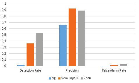
From these results shown in fig. 1 we can see that the Zhou
where a ground truth is provided for the 247th frame. The
et al. provides the best detection rate, moderate precision and
second sequence is named ”Time of Day” and contains a
worst false alarm rate. Ng et al. provides the lowest false alarm
scene with gradual illumination changes. It has 5889 frames
rate, but the worst precision and detection rate. Vemulapalli
where a ground truth is provided for the 1850th frame. The
provides the best precision and moderate detection and false
third sequence is named ”Light Switch” and contains a scene
alarm rates.
with sudden illumination changes. It has 2714 frames where
a ground truth is provided for the 1865th frame. B. Time of Day
From these results shown in fig. 2 we can see that Zhou
B. Metrics has the worst performance; having the worst detection rate,
For the evaluation of the output accuracy we make use of precision and false alarm rate. Ng et al. has a superior
the detection rate (DR), false alarm rate (FAR) and precision precision and false alarm rate as well as a moderate detection
(P) statistics. The formulae for these are provided below: rate. Vemulapalli provides the best detection rate and values
only slightly worse than Ng et al. in regard to precision and
#true positives false alarm rate.
DR = (27)
#true positives + #f alse negatives
C. Light Switch
#f alse positives From these results shown in fig. 3 we can see that Zhou et
F AR = (28)
#f alse positives + #true negatives al. provides the best detection rate, moderate precision and a
#true positives moderate false alarm rate. Ng et al. has the best precision and
P = (29) false alarm rate, but the worst detection rate. Vemulapalli has
#true positives + #f alse positives
a moderate detection rate, but the worst precision and false
Where #true positives is the number of correctly classi- alarm rate.
fied foreground pixels, #true negatives is the number of The poor performance of the solution proposed by Vemu-
correctly classified background pixels, #f alse positives is lapalli is largely due to the fact that the sudden illumination
the number of incorrectly classified foreground pixels and check is not triggered by the video sequence. Hence, the blind
#true negatives is the number of incorrectly classified back- update mechanism for the short-term model is not employed
ground pixels. and the model does not adapt to the new lighting conditions
quickly enough.
C. Selection of Tuning Parameters
Zhou et al. set Rregion = 9, R = 2, N = 4, K = 4,
TP = 0.65, TB = 0.7, αb = αw = β = 0.01, αp = 0.9,
ξ = 2.5 and ε1 = ε2 = 0.2. Zhou et al do not specify
which similarity measure they used; we investigated two, the
L1 Norm and the Square L2 Norm. The latter was determined
to be best by qualitatively comparing their output. Zhou et
al. also did not specify how they initialized the weights of
the model histograms; we investigated two methods: using
a values that decrease linearly and values that decrease ex-
ponentially. The latter was determined to be the best by
Fig. 1: Results of ”Waving Trees” sequence.
qualitative analysis. Using the exponential curve w0 = 0.567,
w1 = 0.321, w2 = 0.103, w3 = 0.011.
Ng et al. set M = 17 and α = 0.1. The value for τ is set
empirically for the dataset at hand. For the experiments they
perform on the PETS 2006 dataset they set τ = 1 × 10⁵ . We
set τ = 1 × 10³ .
Vemulapalli sets W = 250, N = 50 and α = 75%.
However, for the the Waving Trees sequence we set W = 200
and N = 20 since the 247th frame is used for the ground truth.
Vemulapalli does not specify which parameters they used for
the hypersphere radius, r, and the threshold, T . We set r = 1
and T = µ + kσ where µ is the mean and σ is the standard
deviation of the values obtained for M in a frame. k is a Fig. 2: Results of ”Time of Day” sequence.
positive integer which is set to 6.
302a sparse foreground mask that is very accurate for all three
sequences, but has a poor detection rate.
The KDE approach performs well for simple dynamic
backgrounds and scenes that contain gradual illumination
changes. However, the mechanism employed to handle sudden
illumination changes does not work well due to the use of an
unreliable criterion for sudden illumination detection.
VII. F UTURE W ORK
Fig. 3: Results of ”Light Switch” sequence. We plan to further investigate the solution proposed by Ng
et al. and Vemulapalli. Both have potential to be improved
through automatic parameter selection and possibly by in-
tegrating the strengths of all three the solutions that were
investigated.
R EFERENCES
[1] K. K. Ng, S. Srivastava, and E. Delp, “Foreground segmentation with
sudden illumination changes using a shading model and a gaussianity
test,” in Image and Signal Processing and Analysis (ISPA), 7th Interna-
tional Symposium on, September 2011, pp. 236–240.
[2] M. Heikkila and M. Petikainen, “A texture-based method for modelling
the background and detecting moving objects,” IEEE Transactions on
Pattern Analysis and Machine Intelligence, vol. 28, no. 4, pp. 657–662,
2006.
[3] B. Xie, V. Ramesh, and T. Boult, “Sudden illumination change detection
using order consistency,” Image and Vision Computing, vol. 22, no. 2,
pp. 117–125, 2004.
[4] J. Pilet, C. Strecha, and P. Fua, “Making background subtraction robust
to sudden illumination changes,” in Computer Vision–ECCV 2008.
Springer, pp. 567–580, 2008.
[5] J. Li and Z. Miao, “Foreground segmentation for dynamic scenes with
sudden illumination changes,” Image Processing, IET, vol. 6, no. 5, pp.
606–615, July 2012.
Fig. 4: Foreground segmentation masks of proposed solutions. [6] K. Toyama, J. Krumm, B. Brumitt, and B. Meyers, “Wallflower: prin-
The columns correspond to the ”Waving Trees”, ”Time of ciples and practice of background maintenance,” in Computer Vision,
1999. The Proceedings of the Seventh IEEE International Conference
Day” and ”Light Switch” sequences respectively. The first on, vol. 1, pp. 255-261, 1999.
row represents the ground truths while the remaining rows [7] B. Stenger, V. Ramesh, N. Paragios, F. Coetzee, and J. M. Buhmann,
correspond to the outputs of the solutions proposed by Zhou “Topology free hidden markov models: Application to background
modeling,” in Computer Vision, ICCV 2001. Proceedings. Eighth IEEE
et al., Ng et al. and Vemulapalli respectively. International Conference on, vol. 1, pp. 294–301. IEEE, 2001.
[8] X. Zhao, W. He, S. Luo, and L. Zhang, “Mrf-based adaptive approach
for foreground segmentation under sudden illumination change,” in
Information, Communications Signal Processing, 2007 6th International
VI. C ONCLUSION Conference on, pp. 1-4, Dec 2007.
This paper investigates three background modelling tech- [9] Y. Sun and B. Yuan, “Hierarchical gmm to handle sharp changes in
moving object detection,” Electronics Letters, vol. 40, no. 13, pp. 801–
niques that are robust against sudden and gradual illumination 802, 2004.
changes for a single, stationary camera. The first makes [10] Y. Dong, T. Han, and G. N. DeSouza, “Illumination invariant fore-
use of a modified local binary pattern that considers both ground detection using multi-subspace learning,” International journal
of knowledge-based and intelligent engineering systems, vol. 14, no. 1,
spatial texture and colour information. The second uses a pp. 31–41, 2010.
combination of a frame-based Gaussianity Test and a pixel- [11] W. Zhou, Y. Liu, W. Zhang, L. Zhuang, and N. Yu, “Dynamic back-
based Shading Model to handle sudden illumination changes. ground subtraction using spatial-color binary patterns,” in Image and
Graphics (ICIG), 2011 Sixth International Conference on, pp. 314-319,
The third solution is an extension of a popular kernel density Aug 2011.
estimation (KDE) technique from the temporal to spatio- [12] R. Vemulapalli and R. Aravind, “Spatio-temporal nonparametric back-
temporal domain using 9-dimensional data points instead of ground modeling and subtraction,” in Computer Vision Workshops (ICCV
Workshops), 2009 IEEE 12th International Conference on, 1145-1152,
pixel intensity values and a discrete hyperspherical kernel Sept 2009.
instead of a Gaussian kernel. [13] K. Skifstad and R. Jain, “Illumination independent change detection for
A number of experiments were then performed which real world image sequences,” Computer Vision, Graphics, and Image
Processing, vol. 46, no. 3, pp. 387–399, June 1989.
provide a comparison of these techniques in regard to clas- [14] T. W. Ridler and S. Calvard, “Picture thresholding using an iterative
sification accuracy. selection method,” Systems, Man and Cybernetics, IEEE Transactions
The SCBP histogram feature approach performs well for on, vol. 8, no. 8, pp. 630–632, Aug 1978.
[15] A. M. Elgammal, D. Harwood, and L. S. Davis, “Non-parametric
simple dynamic backgrounds, but not for scenes that contain model for background subtraction,” in Proceedings of the 6th European
any type of illumination changes. Conference on Computer Vision-Part II, ser. ECCV ’00. Springer-
The Shading Model and Gaussianity Test approach provides Verlag, 2000, pp. 751–767.
303You can also read