Software Product Line Engineering with Feature Models

Software Product Line Engineering with Feature Models
Danilo Beuche, pure-systems (Danilo.Beuche@pure-systems.com, http://www.pure-systems.com/)
Mark Dalgarno, Software Acumen (mark@software-acumen.com, http://www.software-acumen.com/)

Although the term "Software Product line Engineering" is becoming more widely known, there is still uncertainty
among developers about how it would apply in their own development context. In this article we tackle this problem by
describing the design and automated derivation of the product variants of a Software Product Line using an easy to
understand, practical example.

One increasing trend in software development is the need to develop multiple, similar software products instead of just
a single individual product. There are several reasons for this. Products that are being developed for the international
market must be adapted for different legal or cultural environments, as well as for different languages, and so must
provide adapted user interfaces. Because of cost and time constraints it is not possible for software developers to
develop a new product from scratch for each new customer, and so software reuse must be increased. These types of
problems typically occur in portal or embedded applications, e.g. vehicle control applications [Ste04]. Software Product
Line Engineering (SPLE) offers a solution to these not quite new, but increasingly challenging, problems [Cle01].

The basis of SPLE is the explicit modelling of what is common and what differs between product variants. Feature
Models [Kan90], [Cza00] are frequently used for this. SPLE also includes the design and management of a variable
software architecture and its constituent (software) components.

This article describes how this is done in practice, using the example of a Product Line of meteorological data systems.
Using this example we will show how a Product Line is designed, and how product variants can be derived
automatically.

Software Product Lines
However, before we introduce the example, we'll take a small detour into the basis of SPLE. The main difference from
“normal”, one-of-a-kind software development, is a logical separation between the development of core, reusable
software assets (the platform), and actual applications. During application development, platform software is selected
and configured to meet the specific needs of the application.

The Product Line's commonalities and variabilities are described in the Problem Space. This reflects the desired range
of applications (“product variants”) in the Product Line (the “domain”) and their inter-dependencies. So, when
producing a product variant, the application developer uses the problem space definition to describe the desired
combination of problem variabilities to implement the product variant.

An associated Solution Space describes the constituent assets of the Product Line (the “platform”) and its relation to the
problem space, i.e. rules for how elements of the platform are selected when certain values in the problem space are
selected as part of a product variant. The four-part division resulting from the combination of the problem space and
solution space with domain and application engineering is shown in Figure 1.

                    Figure 1: Overview of SPLE activities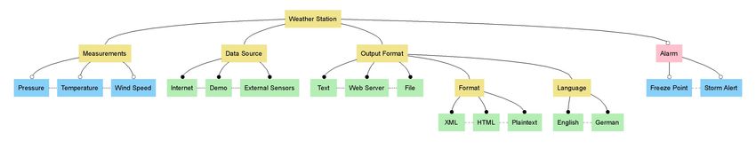

Several different options are available for modelling the information in these four quadrants. The problem space can be
described e.g. with Feature Models, or with a Domain Specific Language (DSL). There are also a number of different
options for modelling the solution space, for example component libraries, DSL compilers, generative programs and
also configuration files. [ Cza00 ].

In the rest of this article we will consider each of these quadrants in turn, beginning with Domain Engineering activities.
We'll first look at modelling the problem space - what is common to, and what differs between, the different product
variants. Then we'll consider one possible approach for realising product variants in the solution space using C++ as an
example. Finally we'll look at how Application Engineering is performed by using the problem and solution space
models to create a product variant. In reality, this linear flow is rarely found in practice. Product Lines usually evolve
continuously, even after the first product variants have been defined and delivered to customers.

Our example Product Line will contain different products for entry and display of meteorological data on a PC. An
initial brainstorming session has led to a set of possible differences (variation points) between possible products:
meteorological data can come from different sensors attached to the PC, fetched from appropriate Internet services or
generated directly by the product for demonstration and test purposes. Data can be output directly from the application,
distributed as HTML or XML through an integrated Web server or regularly written to file on a fixed disk. The
measurements to make can also vary: temperature, air pressure , wind velocity and humidity could all be of interest.
Finally the units of measure could also vary (degrees Celsius vs. Fahrenheit, hPa vs. mmHg, m / s vs. Beaufort).

Modelling the Problem Space
We will now convert the informal, natural-language specification of variability noted above into a formal model, in
order to be able to process it. Specifically, we will use a Feature Model. Feature models are simple, hierarchical models
that capture the commonality and variability of a Product Line. Each relevant characteristic of the problem space
becomes a feature in the model. A definition of the term "feature" is given in Definition 1.

 Features are an abstract concept for describing commonalities and variabilities. What this means precisely needs to be
 decided for each Product Line.

 A feature in this sense is a characteristic of a system relevant for some Stakeholder. Depending on the interest of the
 Stakeholders a feature can be for the example a requirement, a technical function or function group or a non-
 functional (quality) characteristic.
 Definition 1: Features

Feature models have a tree structure, with features forming nodes of the tree. Feature variability is represented by the
arcs and groupings of features. There are four different types of feature groups: “mandatory", “optional", "alternative"
and “or”.

When specifying which features are to be included in a variant the following rules apply: If a parent feature is contained
in a variant,

    ●    all its mandatory child features must be also contained ("n from n"),
    ●    any number of optional features can be included ("m from n, 0 < = m1").

Unfortunately, no single standard has yet been agreed for the graphical notation of feature models. However, in the
literature, the graphical notation of the original FODA method [Ste04] is common. However this is representable with
standard text tools and graph libraries only with difficulty. Therefore in this article a simplified notation has been used.
Alternatives and groups of or features are represented with traverses between the matching features. In this
representation both colour and box connector are used independently to indicate the type of group. Our notation is
shown in Figure 2.

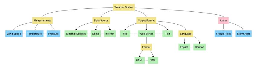
Figure 2: Structure and notation of feature models
Using this notation, our example feature model, with some modifications, is shown in Figure 3:

Figure 3: Feature model for our meteorological Product Line
Each Feature Model has a root feature. Beneath this are three mandatory features – "Measurements", "Data Source" and
"Output Format". Mandatory features will always be included in a product variant if their parent feature is included in
the product variant. Mandatory features are not variable in the true sense, but serve to structure or document their parent
feature in some way. Our example also has alternative features, e.g. "External Sensors", "Demo" and "Internet" for data
sources. All product variants must contain one and only one of these alternatives.

At this stage we can already see one advantage that feature modelling has over a natural-language representation - it
removes ambiguities - e.g. whether an individual variant is able to process data from more than one source. When
taking measurements any combination of measurements is meaningful and at least one measurement source is necessary
for a sensible weather station, to model this we use a group of Or. Usually simple optional features are used, such as the
example of the freezing point alarm. Further improvements can also be made by refining the model hierarchy. So the
strict choice between Web Server output formats - HTML or XML – can be made explicit.

Feature models also support transverse relationships, such as requires and mutually exclusive, in order to model
additional dependencies between features other than those already described. So, in the example model, a selection of
the “Freeze Point” alarm feature is only meaningful in connection with the temperature measurement capability. This
can be modelled by an "Freeze Point" requires "Temperature" relationship (not shown in the figure). However, such
relations should be used sparingly. The more transverse relations there are, the harder it is for a human user to visualize
connections in the model.

When creating a feature model it can be difficult to decide exactly how problem space variabilities are to be represented
in the model. In this case it is best to discuss this further with the customer. It is usually better to base these discussions
around the feature model, since such models are easier for the customer to understand than textual documents and / or
UML models. Formalising customer requirements in this way offers significant advantages later in Product Line
development, since many architectural and implementation decisions can be made on the basis of the variabilities
captured in the feature model. In the example, the use of the output format XML and HTML can be clarified. The
model explicitly defines that the choice of output format is only relevant for Web Server, a format selection is not
possible for File or Text output. However, in the context of a discussion of the feature model it could be decided that
HTML is also desirable for the on-screen (Window) representation and could also be applicable for file storage.

This results in the modified feature model shown in Figure 4.

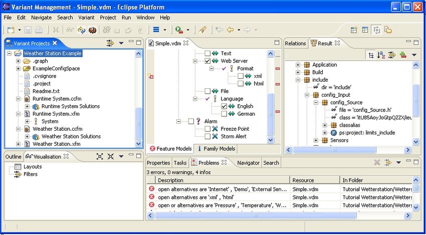
Figure 4: Enhanced Feature Model for our meteorological Product Line
We have added “Plaintext” to the existing features; this was implicitly assumed for output to the screen or to a file. We
have modelled the mutual exclusion of XML and screen display (“Text”) using a (transverse) relationship between
these features (not shown).

The previous discussion describes the basic feature model approach commonly found in the literature, but a number of
people have extended this basic approach. To complement the so-called hard relations between features (requires and
conflicts) the weakened forms recommends and discourages have been added to many feature model dialects.
pure::variants [pure], the variant management tool used for modelling the example in this article, also supports the
association of named attributes with features. This allows numeric values or enumerated values to be conveniently
associated with features e.g. the wind force required to activate the storm alarm could be represented as a "Threshold"
attribute of the feature "Storm Alert".

An important and difficult issue in the creation of feature models is deciding which problem space features to represent.
In the example model it is not possible to make a choice from the available hardware sensor types (e.g. use of a PR1003
or a PR2005 sensor for pressure). So, when specifying a variant, the user does not have direct influence on the selection
of sensor types. These are determined when modelling the solution space. If the choice of different sensor types for
measuring pressure is a major criterion for the customer / users, then appropriate options would have to be included in
the feature model. This means that the features in the problem space are not a 1:1-illustration of the possibilities in the
solution space, but only represent the (variable) characteristics relevant for the users of the Product Line. Feature
models are a user-oriented (or marketing-oriented) representation of the problem space, not the solution space.

After creating the problem space model we can use it to perform some initial analysis. For example, we can now
calculate the upper limit on the number of possible variants in our example Product Line. In this case we have 1,512
variants (the model in Figure 2 only has 612 variants). For such a small number of variants the listing of all possible
variants can be meaningful. However, the number of variants is usually too high to make practical use of such an
enumeration.

Modelling the Solution Space
In order to implement the solution space using a suitable variable architecture, we must take account of other factors
beyond the variability model of the problem space. These include common characteristics of all variants of the problem
space that are not modelled in the feature model, as well as other constraints that limit the solution space.

These typically include the programming languages that can be used, the development environment and the application
deployment environment(s). Different factors affect the choice of mechanisms to be used for converting from variation
points in the solution space. These include the available development tools, the required performance and the available
(computing) resources, as well as time and money. For example, use of configuration files can reduce development time
for a project, if users can administer their own configurations. In other cases, using preprocessor directives (#ifdef) for
conditional compilation can be appropriate, e.g. if smaller program sizes are required.

There are many possibilities for implementation of the solution space. Very simple variant-specific model
transformations can be made with model-driven software development (MDSD) tools by including information from
feature models in the Model-Transformation process. [Voel05] gives an example using the openArchitectureware
model transformer. Aspect-oriented programming (AOP) can also be used as a means for the efficient conversion of
variabilities in the solution space. Product Lines can also be implemented naturally using "classical" means such as
procedural or object-oriented languages.

Designing a variable architecture
A Product Line architecture will only rarely result directly from the structure of the problem space model. The solution
space which can be implemented should support the variability of the problem space, but won't necessarily be a 1:1
correspondence with the architecture. The mapping of variabilities can take place in various ways.

In the example Product Line we will use a simple object-oriented design concept implemented in C++ . A majority of
the variability is then resolved at compile-time or link-time; runtime variability is only used if it is absolutely necessary.
Such solutions are frequently used in practice, particularly in embedded systems.

The choice of which tools to use for automating the configuration and / or production of a variant plays a substantial
role in the design and implementation of the solution space. The range of variability, the complexity of relations
between problem space features and solution constituents, the number and frequency of variant production, the size and
experience of the development team and many further factors play a role. In simple cases the variant can be produced
by hand, but automated tools in the form of Excel and / or small configuration scripts, and also model transformers,
code generators or variant management systems will speed production.

For modelling and mapping of the solution space variability we use pure::variants [pure] and its integrated model
transformation. This uses a Family Model to model the solution space, to associate solution space elements with
problem space features, and to support the automatic selection of solution space elements when constructing a product
variant.

Family models have a hierarchical structure, consisting of logical items of the solution architecture, e.g. components,
classes and objects. These logical items can be augmented with information about "real" solution elements such as
source code files, in order to enable automatic production of a solution from a valid feature model configuration (more
on this later). For each family model element a rule is created to link it to the solution space. For example, the Web
Server implementation component is only included if the Web Server feature has been selected from the problem space.
To achieve this, a hasFeature('Web Server') rule is attached to the "Web Server" component . Any item below “Web
Server” in the Family model can only be included in the solution if the corresponding Web Server feature is selected.

A pure::variants screen shot showing part of the solution space is shown in Figure 5.

Figure 5: pure::variants screen shot - solution space fragment shown at right
In our example, an architectural variation point arises, among other possibilities, in the area of data output. Each output
format can be implemented with an object of a format-specific output class. Thus in the case of HTML output, an object
of type HtmlOutput is instantiated, and with XML output, an XmlOutput object. There would also be the possibility
here of instantiating an appropriate object at runtime using a Strategy pattern. However, since the feature model
designates only the use of alternative output formats, the variability can be resolved at compile-time and a suitable
object can be instantiated using code generation for example.

In our example solution space a lookup in a text database is used to support multiple natural languages. The choice of
which database to use is made at compile-time depending on the desired language. No difference in solution
architectures can be detected between two variants that differ only in the target language. Here the variation point is

embedded in the data level of the implementation.

In many cases managing variable solutions only at the architectural level is insufficient. As has already been mentioned
above, we must also support variation points at the implementation level, i.e. in our case at the C++ source code level.
This is necessary to support automated product derivation. The constituents of a solution on the implementation level,
like source code files or configuration files which can be generated, can also be entered in the family model and
associated with selection rules.

So the existence of the Web Server component in a product variant is denoted using a #define preprocessor directive in
a configuration Header file. In addition, an appropriate abstract variation point variable "WEB SERVER" must first be
created of the type ps:variable in the family model. The value of this variable is determined by a Value attribute. In our
case this value is always 1 if the variable is contained in the product variant. An item of type ps:flagfile can now be
assigned to this abstract variable. This item also possesses attributes (file, flag), which are used during the
transformation of the model into "real" code. The meaning of the attributes is determined by the transformation
selected in the generation step . Here we use the standard pure::variants transformation for C / C++ programs, which
produces a C-preprocessor #define- Flags in the file defined by file from these specifications.

Separating the logical variation point from the solution makes it very simple to manage changes to the solution space.
For example, if the same variation point requires an entry in a Makefile, this could be achieved with the definition of a
further source element, of the type ps:makefile, below the variation point "WEB SERVER".

Deriving product variants
The family model captures both the structure of the solution space with its variation points and the connection of
solution and problem space. Not only is the separation of these two spaces important, but also the direction of the
connection, since problem space models in most cases are much more stable than solution spaces; the linkage of the
solution space to the problem space is more meaningful than the selection of solution items by rules in the problem
space. This also increases the potential for reuse, since problem space models can simply be combined with other (new,
better, faster) solutions.

Now we have all the information needed to create an individual product variant. The first step is to determine a valid
selection of characteristics from the feature model. In the case of pure::variants, the user is guided towards a valid and
complete feature selection. Once a valid selection is found, the specified feature list as well as the family model serve as
input for the production of a variant model. Then, as is described above, the rules of the individual model items are
checked. Only items that have their rules satisfied are included in the finished solution.

Open Issues in SPLE
So far we have highlighted some of the most common issues that will be encountered when working with Software
Product Lines. In this section we highlight some additional issues.

Even with visualization support from specialist tools such as pure::variants the visual representation of very complex
model structures is a not a completely solved problem. Larger feature models can have several hundred features and the
solution space can have several thousands or more constituents. Thus it can be hard to understand the implications of
modifications to these models just through use of model diagrams.

Issues around Product Line evolution are also very important. Evolution must be managed since changes that positively
affect one or more variants could have a negative effect on other variants and these issues may only show up when
variants are produced long after the changes have been implemented.

Finally, testing a Product Line also represents a significant challenge. Most Product Lines offer more potential
variability than is in use at any one time, and testing all possible variants is usually impossible and in some cases a
waste of time. Testing just those variants that are produced is already a difficult problem where there is a high number
of variants. However, it is still necessary to co-ordinate testing with variant production in some way. One approach is
to create test asset variants as one does for the (software) solution space variants – effectively creating a parallel test
solution space that is driven from the Feature model. Reduction of test effort is still an open issue though for many
Product Lines.

Closing Remarks
The example presented in this article shows how the variability of the problem space of a Product Line can be described
very simply using feature models. The automated production of solution variants is the logical next step, for which we
have shown one example. In this example we have highlighted some of the approaches and issues that need to be

considered when using Software Product Lines. These are covered in more depth in [Bos00], a standard work on
Software Product Lines, for example.

The authors also welcome comments and questions on any aspect of Software Product Lines Engineering.

References and Links
[Bos00] J. Bosch, Design and Use of Software Architectures: Adopting and Evolving a Product Line Approach,
Addison-Wesley, 2000

[Cle01] P. Clements, L Northrop, Software Product Lines: Practices & Patterns, Addison-Wesley 2001 (see also
www.sei.cmu.edu/productlines/framework.html

[Cza00] K. Czarnecki, U.W. Eisenecker, Generative Programming: Methods, Tools, and Applications, Addison-
Wesley, 2000

[Kan90] K. Kang, et al., Feature Oriented Domain Analysis (FODA) Feasibility Study, Technical report CMU/SEI-90-
TR-021, Software Engineering Institute, Carnegie Mellon University, 1990

[pure] pure system GmbH website: www.pure-systems.com

[Ste04] M. Steger et al., Introducing PLA RK Bosch Gasoline of System: Experiences and Practices, in: Proc. of the
Software Product Line Conf. 2004, S. 34-50

[Voel05] M. Voelter, Variantenmanagement in the context of MDSD, in: JavaSpektrum 5/05